
Introduction to Data Structures and Algorithms

Data Structure is a way of collecting and organising data in such a way that we can perform orations on these data in an effective way. Data Structures is about rendering data elements in terms of some relationship, for better organization and storage. For example, we have some data which has, player's name "Virat" and age 26. Here "Virat" is of String data type and 26 is of integer data type.
We can organize this data as a record like Player record, which will have both player's name and age in it. Now we can collect and store player's records in a file or database as a data structure. For example: "Dhoni" 30, "Gambhir" 31, "Sehwag" 33
If you are aware of Object Oriented programming concepts, then a class also does the same thing, it collects different type of data under one single entity. The only difference being, data structures provides for techniques to access and manipulate data efficiently.
In simple language, Data Structures are structures programmed to store ordered data, so that various operations can be performed on it easily. It represents the knowledge of data to be organized in memory. It should be designed and implemented in such a way that it reduces the complexity and increases the efficiency.
Basic types of Data Structures
As we have discussed above, anything that can store data can be called as a data structure, hence Integer, Float, Boolean, Char etc, all are data structures. They are known as Primitive Data Structures.
Then we also have some complex Data Structures, which are used to store large and connected data. Some example of Abstract Data Structure are :
- Linked List
- Tree
- Graph
- Stack, Queue etc.
All these data structures allow us to perform different operations on data. We select these data structures based on which type of operation is required. We will look into these data structures in more details in our later lessons.

The data structures can also be classified on the basis of the following characteristics:
| Characterstic | Description |
|---|---|
| Linear | In Linear data structures,the data items are arranged in a linear sequence. Example: Array |
| Non-Linear | In Non-Linear data structures,the data items are not in sequence. Example: Tree, Graph |
| Homogeneous | In homogeneous data structures,all the elements are of same type. Example: Array |
| Non-Homogeneous | In Non-Homogeneous data structure, the elements may or may not be of the same type. Example: Structures |
| Static | Static data structures are those whose sizes and structures associated memory locations are fixed, at compile time. Example: Array |
| Dynamic | Dynamic structures are those which expands or shrinks depending upon the program need and its execution. Also, their associated memory locations changes. Example: Linked List created using pointers |
What is an Algorithm ?
An algorithm is a finite set of instructions or logic, written in order, to accomplish a certain predefined task. Algorithm is not the complete code or program, it is just the core logic(solution) of a problem, which can be expressed either as an informal high level description as pseudocode or using a flowchart.
Every Algorithm must satisfy the following properties:
- Input- There should be 0 or more inputs supplied externally to the algorithm.
- Output- There should be atleast 1 output obtained.
- Definiteness- Every step of the algorithm should be clear and well defined.
- Finiteness- The algorithm should have finite number of steps.
- Correctness- Every step of the algorithm must generate a correct output.
An algorithm is said to be efficient and fast, if it takes less time to execute and consumes less memory space. The performance of an algorithm is measured on the basis of following properties :
- Time Complexity
- Space Complexity
Space Complexity
Its the amount of memory space required by the algorithm, during the course of its execution. Space complexity must be taken seriously for multi-user systems and in situations where limited memory is available.
An algorithm generally requires space for following components :
- Instruction Space: Its the space required to store the executable version of the program. This space is fixed, but varies depending upon the number of lines of code in the program.
- Data Space: Its the space required to store all the constants and variables(including temporary variables) value.
- Environment Space: Its the space required to store the environment information needed to resume the suspended function.
To learn about Space Complexity in detail, jump to the Space Complexity tutorial.
Time Complexity
Time Complexity is a way to represent the amount of time required by the program to run till its completion. It's generally a good practice to try to keep the time required minimum, so that our algorithm completes it's execution in the minimum time possible. We will study about Time Complexity in details in later sections.
NOTE: Before going deep into data structure, you should have a good knowledge of programming either in C or in C++ or Java or Python etc.
Asymptotic Notations
When it comes to analysing the complexity of any algorithm in terms of time and space, we can never provide an exact number to define the time required and the space required by the algorithm, instead we express it using some standard notations, also known as Asymptotic Notations.
When we analyse any algorithm, we generally get a formula to represent the amount of time required for execution or the time required by the computer to run the lines of code of the algorithm, number of memory accesses, number of comparisons, temporary variables occupying memory space etc. This formula often contains unimportant details that don't really tell us anything about the running time.
Let us take an example, if some algorithm has a time complexity of T(n) = (n2 + 3n + 4), which is a quadratic equation. For large values of n, the 3n + 4 part will become insignificant compared to the n2 part.
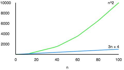
For n = 1000, n2 will be 1000000 while 3n + 4 will be 3004.
Also, When we compare the execution times of two algorithms the constant coefficients of higher order terms are also neglected.
An algorithm that takes a time of 200n2 will be faster than some other algorithm that takes n3 time, for any value of n larger than 200. Since we're only interested in the asymptotic behavior of the growth of the function, the constant factor can be ignored too.
What is Asymptotic Behaviour
The word Asymptotic means approaching a value or curve arbitrarily closely (i.e., as some sort of limit is taken).
Remember studying about Limits in High School, this is the same.
The only difference being, here we do not have to find the value of any expression where n is approaching any finite number or infinity, but in case of Asymptotic notations, we use the same model to ignore the constant factors and insignificant parts of an expression, to device a better way of representing complexities of algorithms, in a single coefficient, so that comparison between algorithms can be done easily.
Let's take an example to understand this:
If we have two algorithms with the following expressions representing the time required by them for execution, then:
Expression 1: (20n2 + 3n - 4)
Expression 2: (n3 + 100n - 2)
Now, as per asymptotic notations, we should just worry about how the function will grow as the value of n(input) will grow, and that will entirely depend on n2 for the Expression 1, and on n3 for Expression 2. Hence, we can clearly say that the algorithm for which running time is represented by the Expression 2, will grow faster than the other one, simply by analysing the highest power coeeficient and ignoring the other constants(20 in 20n2) and insignificant parts of the expression(3n - 4 and 100n - 2).
The main idea behind casting aside the less important part is to make things manageable.
All we need to do is, first analyse the algorithm to find out an expression to define it's time requirements and then analyse how that expression will grow as the input(n) will grow.
Types of Asymptotic Notations
We use three types of asymptotic notations to represent the growth of any algorithm, as input increases:
- Big Theta (Θ)
- Big Oh(O)
- Big Omega (Ω)
Tight Bounds: Theta
When we say tight bounds, we mean that the time compexity represented by the Big-Θ notation is like the average value or range within which the actual time of execution of the algorithm will be.
For example, if for some algorithm the time complexity is represented by the expression 3n2 + 5n, and we use the Big-Θ notation to represent this, then the time complexity would be Θ(n2), ignoring the constant coefficient and removing the insignificant part, which is 5n.
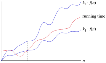
Here, in the example above, complexity of Θ(n2) means, that the avaerage time for any input n will remain in between, k1 * n2 and k2 * n2, where k1, k2 are two constants, therby tightly binding the expression rpresenting the growth of the algorithm.
Upper Bounds: Big-O
This notation is known as the upper bound of the algorithm, or a Worst Case of an algorithm.
It tells us that a certain function will never exceed a specified time for any value of input n.
The question is why we need this representation when we already have the big-Θ notation, which represents the tightly bound running time for any algorithm. Let's take a small example to understand this.
Consider Linear Search algorithm, in which we traverse an array elements, one by one to search a given number.
In Worst case, starting from the front of the array, we find the element or number we are searching for at the end, which will lead to a time complexity of n, where n represents the number of total elements.
But it can happen, that the element that we are searching for is the first element of the array, in which case the time complexity will be 1.
Now in this case, saying that the big-Θ or tight bound time complexity for Linear search is Θ(n), will mean that the time required will always be related to n, as this is the right way to represent the average time complexity, but when we use the big-O notation, we mean to say that the time complexity is O(n), which means that the time complexity will never exceed n, defining the upper bound, hence saying that it can be less than or equal to n, which is the correct representation.
This is the reason, most of the time you will see Big-O notation being used to represent the time complexity of any algorithm, because it makes more sense.
Lower Bounds: Omega
Big Omega notation is used to define the lower bound of any algorithm or we can say the best case of any algorithm.
This always indicates the minimum time required for any algorithm for all input values, therefore the best case of any algorithm.
In simple words, when we represent a time complexity for any algorithm in the form of big-Ω, we mean that the algorithm will take atleast this much time to cmplete it's execution. It can definitely take more time than this too.
Space Complexity of Algorithms
Whenever a solution to a problem is written some memory is required to complete. For any algorithm memory may be used for the following:
- Variables (This include the constant values, temporary values)
- Program Instruction
- Execution
Space complexity is the amount of memory used by the algorithm (including the input values to the algorithm) to execute and produce the result.
Sometime Auxiliary Space is confused with Space Complexity. But Auxiliary Space is the extra space or the temporary space used by the algorithm during it's execution.
Space Complexity = Auxiliary Space + Input space
Memory Usage while Execution
While executing, algorithm uses memory space for three reasons:
- Instruction Space
It's the amount of memory used to save the compiled version of instructions.
- Environmental Stack
Sometimes an algorithm(function) may be called inside another algorithm(function). In such a situation, the current variables are pushed onto the system stack, where they wait for further execution and then the call to the inside algorithm(function) is made.
For example, If a function
A()calls functionB()inside it, then all th variables of the functionA()will get stored on the system stack temporarily, while the functionB()is called and executed inside the funcitonA(). - Data Space
Amount of space used by the variables and constants.
But while calculating the Space Complexity of any algorithm, we usually consider only Data Space and we neglect the Instruction Space and Environmental Stack.
Calculating the Space Complexity
For calculating the space complexity, we need to know the value of memory used by different type of datatype variables, which generally varies for different operating systems, but the method for calculating the space complexity remains the same.
| Type | Size |
|---|---|
| bool, char, unsigned char, signed char, __int8 | 1 byte |
| __int16, short, unsigned short, wchar_t, __wchar_t | 2 bytes |
| float, __int32, int, unsigned int, long, unsigned long | 4 bytes |
| double, __int64, long double, long long | 8 bytes |
Now let's learn how to compute space complexity by taking a few examples:
{
    int z = a + b + c;
    return(z);
}
In the above expression, variables a, b, c and z are all integer types, hence they will take up 4 bytes each, so total memory requirement will be (4(4) + 4) = 20 bytes, this additional 4 bytes is for return value. And because this space requirement is fixed for the above example, hence it is called Constant Space Complexity.
Let's have another example, this time a bit complex one,
// n is the length of array a[]
int sum(int a[], int n)
{
	int x = 0;		// 4 bytes for x
	for(int i = 0; i < n; i++)	// 4 bytes for i
	{
	    x  = x + a[i];
	}
	return(x);
}- In the above code,
4*nbytes of space is required for the arraya[]elements. - 4 bytes each for
x,n,iand the return value.
Hence the total memory requirement will be (4n + 12), which is increasing linearly with the increase in the input value n, hence it is called as Linear Space Complexity.
Similarly, we can have quadratic and other complex space complexity as well, as the complexity of an algorithm increases.
But we should always focus on writing algorithm code in such a way that we keep the space complexity minimum.
Time Complexity of Algorithms
For any defined problem, there can be N number of solution. This is true in general. If I have a problem and I discuss about the problem with all of my friends, they will all suggest me different solutions. And I am the one who has to decide which solution is the best based on the circumstances.
Similarly for any problem which must be solved using a program, there can be infinite number of solutions. Let's take a simple example to understand this. Below we have two different algorithms to find square of a number(for some time, forget that square of any number n is n*n):
One solution to this problem can be, running a loop for n times, starting with the number n and adding n to it, every time.
/*
    we have to calculate the square of n
*/
for i=1 to n
    do n = n + n
// when the loop ends n will hold its square
return n
Or, we can simply use a mathematical operator * to find the square.
/*
    we have to calculate the square of n
*/
return n*n
In the above two simple algorithms, you saw how a single problem can have many solutions. While the first solution required a loop which will execute for n number of times, the second solution used a mathematical operator * to return the result in one line. So which one is the better approach, of course the second one.
What is Time Complexity?
Time complexity of an algorithm signifies the total time required by the program to run till its completion.
The time complexity of algorithms is most commonly expressed using the big O notation. It's an asymptotic notation to represent the time complexity. We will study about it in detail in the next tutorial.
Time Complexity is most commonly estimated by counting the number of elementary steps performed by any algorithm to finish execution. Like in the example above, for the first code the loop will run n number of times, so the time complexity will be n atleast and as the value of n will increase the time taken will also increase. While for the second code, time complexity is constant, because it will never be dependent on the value of n, it will always give the result in 1 step.
And since the algorithm's performance may vary with different types of input data, hence for an algorithm we usually use the worst-case Time complexity of an algorithm because that is the maximum time taken for any input size.
Calculating Time Complexity
Now lets tap onto the next big topic related to Time complexity, which is How to Calculate Time Complexity. It becomes very confusing some times, but we will try to explain it in the simplest way.
Now the most common metric for calculating time complexity is Big O notation. This removes all constant factors so that the running time can be estimated in relation to N, as N approaches infinity. In general you can think of it like this :
statement;
Above we have a single statement. Its Time Complexity will be Constant. The running time of the statement will not change in relation to N.
for(i=0; i < N; i++)
{
    statement;
}
The time complexity for the above algorithm will be Linear. The running time of the loop is directly proportional to N. When N doubles, so does the running time.
for(i=0; i < N; i++)
{
    for(j=0; j < N;j++)
    {
    statement;
    }
}
This time, the time complexity for the above code will be Quadratic. The running time of the two loops is proportional to the square of N. When N doubles, the running time increases by N * N.
while(low <= high)
{
    mid = (low + high) / 2;
    if (target < list[mid])
        high = mid - 1;
    else if (target > list[mid])
        low = mid + 1;
    else break;
}
This is an algorithm to break a set of numbers into halves, to search a particular field(we will study this in detail later). Now, this algorithm will have a Logarithmic Time Complexity. The running time of the algorithm is proportional to the number of times N can be divided by 2(N is high-low here). This is because the algorithm divides the working area in half with each iteration.
void quicksort(int list[], int left, int right)
{
    int pivot = partition(list, left, right);
    quicksort(list, left, pivot - 1);
    quicksort(list, pivot + 1, right);
}
Taking the previous algorithm forward, above we have a small logic of Quick Sort(we will study this in detail later). Now in Quick Sort, we divide the list into halves every time, but we repeat the iteration N times(where N is the size of list). Hence time complexity will be N*log( N ). The running time consists of N loops (iterative or recursive) that are logarithmic, thus the algorithm is a combination of linear and logarithmic.
NOTE: In general, doing something with every item in one dimension is linear, doing something with every item in two dimensions is quadratic, and dividing the working area in half is logarithmic.
Types of Notations for Time Complexity
Now we will discuss and understand the various notations used for Time Complexity.- Big Oh denotes "fewer than or the same as" <expression> iterations.
- Big Omega denotes "more than or the same as" <expression> iterations.
- Big Theta denotes "the same as" <expression> iterations.
- Little Oh denotes "fewer than" <expression> iterations.
- Little Omega denotes "more than" <expression> iterations.
Understanding Notations of Time Complexity with Example
O(expression) is the set of functions that grow slower than or at the same rate as expression. It indicates the maximum required by an algorithm for all input values. It represents the worst case of an algorithm's time complexity.
Omega(expression) is the set of functions that grow faster than or at the same rate as expression. It indicates the minimum time required by an algorithm for all input values. It represents the best case of an algorithm's time complexity.
Theta(expression) consist of all the functions that lie in both O(expression) and Omega(expression). It indicates the average bound of an algorithm. It represents the average case of an algorithm's time complexity.
Suppose you've calculated that an algorithm takes f(n) operations, where,
f(n) = 3*n^2 + 2*n + 4. // n^2 means square of nSince this polynomial grows at the same rate as n2, then you could say that the function f lies in the set Theta(n2). (It also lies in the sets O(n2) and Omega(n2) for the same reason.)
The simplest explanation is, because Theta denotes the same as the expression. Hence, as f(n) grows by a factor of n2, the time complexity can be best represented as Theta(n2).
Introduction to Sorting
Sorting is nothing but arranging the data in ascending or descending order. The term sorting came into picture, as humans realised the importance of searching quickly.
There are so many things in our real life that we need to search for, like a particular record in database, roll numbers in merit list, a particular telephone number in telephone directory, a particular page in a book etc. All this would have been a mess if the data was kept unordered and unsorted, but fortunately the concept of sorting came into existence, making it easier for everyone to arrange data in an order, hence making it easier to search.
Sorting arranges data in a sequence which makes searching easier.
Sorting Efficiency
If you ask me, how will I arrange a deck of shuffled cards in order, I would say, I will start by checking every card, and making the deck as I move on.
It can take me hours to arrange the deck in order, but that's how I will do it.
Well, thank god, computers don't work like this.
Since the beginning of the programming age, computer scientists have been working on solving the problem of sorting by coming up with various different algorithms to sort data.
The two main criterias to judge which algorithm is better than the other have been:
- Time taken to sort the given data.
- Memory Space required to do so.
Different Sorting Algorithms
There are many different techniques available for sorting, differentiated by their efficiency and space requirements. Following are some sorting techniques which we will be covering in next few tutorials.
- Bubble Sort
- Insertion Sort
- Selection Sort
- Quick Sort
- Merge Sort
- Heap Sort
Although it's easier to understand these sorting techniques, but still we suggest you to first learn about Space complexity, Time complexity and the searching algorithms, to warm up your brain for sorting algorithms.
Bubble Sort Algorithm
Bubble Sort is a simple algorithm which is used to sort a given set of n elements provided in form of an array with n number of elements. Bubble Sort compares all the element one by one and sort them based on their values.
If the given array has to be sorted in ascending order, then bubble sort will start by comparing the first element of the array with the second element, if the first element is greater than the second element, it will swap both the elements, and then move on to compare the second and the third element, and so on.
If we have total n elements, then we need to repeat this process for n-1 times.
It is known as bubble sort, because with every complete iteration the largest element in the given array, bubbles up towards the last place or the highest index, just like a water bubble rises up to the water surface.
Sorting takes place by stepping through all the elements one-by-one and comparing it with the adjacent element and swapping them if required.
Implementing Bubble Sort Algorithm
Following are the steps involved in bubble sort(for sorting a given array in ascending order):
- Starting with the first element(index = 0), compare the current element with the next element of the array.
- If the current element is greater than the next element of the array, swap them.
- If the current element is less than the next element, move to the next element. Repeat Step 1.
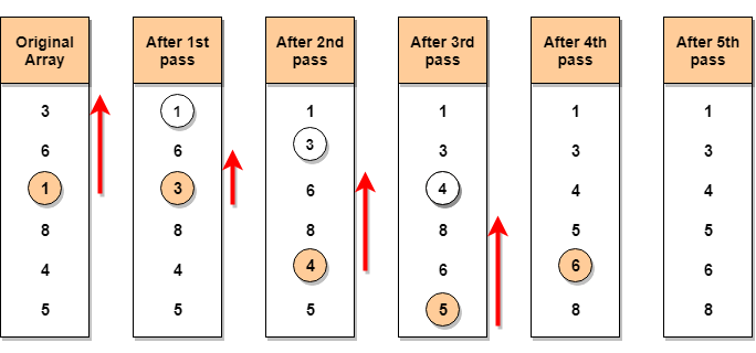
Let's consider an array with values {5, 1, 6, 2, 4, 3}
Below, we have a pictorial representation of how bubble sort will sort the given array.
So as we can see in the representation above, after the first iteration, 6 is placed at the last index, which is the correct position for it.
Similarly after the second iteration, 5 will be at the second last index, and so on.
Time to write the code for bubble sort:
// below we have a simple C program for bubble sort
#include <stdio.h>
void bubbleSort(int arr[], int n)
{
int i, j, temp;
for(i = 0; i < n; i++)
{
for(j = 0; j < n-i-1; j++)
{
if( arr[j] > arr[j+1])
{
// swap the elements
temp = arr[j];
arr[j] = arr[j+1];
arr[j+1] = temp;
}
}
}
// print the sorted array
printf("Sorted Array: ");
for(i = 0; i < n; i++)
{
printf("%d ", arr[i]);
}
}
int main()
{
int arr[100], i, n, step, temp;
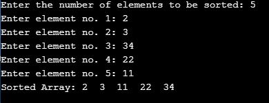
// ask user for number of elements to be sorted
printf("Enter the number of elements to be sorted: ");
scanf("%d", &n);
// input elements if the array
for(i = 0; i < n; i++)
{
printf("Enter element no. %d: ", i+1);
scanf("%d", &arr[i]);
}
// call the function bubbleSort
bubbleSort(arr, n);
return 0;
}Although the above logic will sort an unsorted array, still the above algorithm is not efficient because as per the above logic, the outer for loop will keep on executing for 6 iterations even if the array gets sorted after the second iteration.
So, we can clearly optimize our algorithm.
Optimized Bubble Sort Algorithm
To optimize our bubble sort algorithm, we can introduce a flag to monitor whether elements are getting swapped inside the inner for loop.
Hence, in the inner for loop, we check whether swapping of elements is taking place or not, everytime.
If for a particular iteration, no swapping took place, it means the array has been sorted and we can jump out of the for loop, instead of executing all the iterations.
Let's consider an array with values {11, 17, 18, 26, 23}
Below, we have a pictorial representation of how the optimized bubble sort will sort the given array.
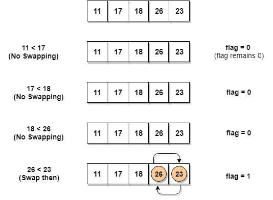
As we can see, in the first iteration, swapping took place, hence we updated our flag value to 1, as a result, the execution enters the for loop again. But in the second iteration, no swapping will occur, hence the value of flag will remain 0, and execution will break out of loop.
// below we have a simple C program for bubble sort
#include <stdio.h>

void bubbleSort(int arr[], int n)
{
    int i, j, temp, flag=0;
    for(i = 0; i < n; i++)
    {
        for(j = 0; j < n-i-1; j++)
        {
            // introducing a flag to monitor swapping
            if( arr[j] > arr[j+1])
            {
                // swap the elements
                temp = arr[j];
                arr[j] = arr[j+1];
                arr[j+1] = temp;
                // if swapping happens update flag to 1
                flag = 1;
            }
        }
        // if value of flag is zero after all the iterations of inner loop
        // then break out
        if(flag==0)
        {
            break;
        }
    }

    // print the sorted array
    printf("Sorted Array: ");
    for(i = 0; i < n; i++)
    {
        printf("%d  ", arr[i]);
    }
}

int main()
{
    int arr[100], i, n, step, temp;
    // ask user for number of elements to be sorted
    printf("Enter the number of elements to be sorted: ");
    scanf("%d", &n);
    // input elements if the array
    for(i = 0; i < n; i++)
    {
        printf("Enter element no. %d: ", i+1);
        scanf("%d", &arr[i]);
    }
    // call the function bubbleSort
    bubbleSort(arr, n);

    return 0;
}
In the above code, in the function bubbleSort, if for a single complete cycle of j iteration(inner for loop), no swapping takes place, then flag will remain 0 and then we will break out of the for loops, because the array has already been sorted.
Complexity Analysis of Bubble Sort
In Bubble Sort, n-1 comparisons will be done in the 1st pass, n-2 in 2nd pass, n-3 in 3rd pass and so on. So the total number of comparisons will be,
(n-1) + (n-2) + (n-3) + ..... + 3 + 2 + 1 Sum = n(n-1)/2 i.e O(n2)
Hence the time complexity of Bubble Sort is O(n2).
The main advantage of Bubble Sort is the simplicity of the algorithm.
The space complexity for Bubble Sort is O(1), because only a single additional memory space is required i.e. for temp variable.
Also, the best case time complexity will be O(n), it is when the list is already sorted.
Following are the Time and Space complexity for the Bubble Sort algorithm.
- Worst Case Time Complexity [ Big-O ]: O(n2)
- Best Case Time Complexity [Big-omega]: O(n)
- Average Time Complexity [Big-theta]: O(n2)
- Space Complexity: O(1)
Selection Sort Algorithm
Selection sort is conceptually the most simplest sorting algorithm. This algorithm will first find the smallest element in the array and swap it with the element in the first position, then it will find the second smallest element and swap it with the element in the second position, and it will keep on doing this until the entire array is sorted.
It is called selection sort because it repeatedly selects the next-smallest element and swaps it into the right place.
How Selection Sort Works?
Following are the steps involved in selection sort(for sorting a given array in ascending order):
- Starting from the first element, we search the smallest element in the array, and replace it with the element in the first position.
- We then move on to the second position, and look for smallest element present in the subarray, starting from index
1, till the last index. - We replace the element at the second position in the original array, or we can say at the first position in the subarray, with the second smallest element.
- This is repeated, until the array is completely sorted.
Let's consider an array with values
{3, 6, 1, 8, 4, 5}Below, we have a pictorial representation of how selection sort will sort the given array.
In the first pass, the smallest element will be
1, so it will be placed at the first position.Then leaving the first element, next smallest element will be searched, from the remaining elements. We will get
3as the smallest, so it will be then placed at the second position.Then leaving
1and3(because they are at the correct position), we will search for the next smallest element from the rest of the elements and put it at third position and keep doing this until array is sorted.Finding Smallest Element in a subarray
In selection sort, in the first step, we look for the smallest element in the array and replace it with the element at the first position. This seems doable, isn't it?
Consider that you have an array with following values
{3, 6, 1, 8, 4, 5}. Now as per selection sort, we will start from the first element and look for the smallest number in the array, which is1and we will find it at the index2. Once the smallest number is found, it is swapped with the element at the first position.Well, in the next iteration, we will have to look for the second smallest number in the array. How can we find the second smallest number? This one is tricky?
If you look closely, we already have the smallest number/element at the first position, which is the right position for it and we do not have to move it anywhere now. So we can say, that the first element is sorted, but the elements to the right, starting from index
1are not.So, we will now look for the smallest element in the subarray, starting from index
1, to the last index.Confused? Give it time to sink in.
After we have found the second smallest element and replaced it with element on index
1(which is the second position in the array), we will have the first two positions of the array sorted.Then we will work on the subarray, starting from index
2now, and again looking for the smallest element in this subarray.Implementing Selection Sort Algorithm
In the C program below, we have tried to divide the program into small functions, so that it's easier fo you to understand which part is doing what.
There are many different ways to implement selection sort algorithm, here is the one that we like:
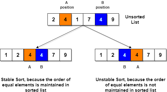
// C program implementing Selection Sort
# include <stdio.h>

// function to swap elements at the given index values
void swap(int arr[], int firstIndex, int secondIndex)
{
    int temp;
    temp = arr[firstIndex];
    arr[firstIndex] = arr[secondIndex];
    arr[secondIndex] = temp;
}

// function to look for smallest element in the given subarray
int indexOfMinimum(int arr[], int startIndex, int n)
{
    int minValue = arr[startIndex];
    int minIndex = startIndex;

    for(int i = minIndex + 1; i < n; i++) {
        if(arr[i] < minValue)
        {
            minIndex = i;
            minValue = arr[i];
        }
    }
    return minIndex;
}

void selectionSort(int arr[], int n)
{
    for(int i = 0; i < n; i++)
    {
        int index = indexOfMinimum(arr, i, n);
        swap(arr, i, index);
    }

}

void printArray(int arr[], int size)
{
    int i;
    for(i = 0; i < size; i++)
    {
        printf("%d ", arr[i]);
    }
    printf("\n");
}

int main()
{
    int arr[] = {46, 52, 21, 22, 11};
    int n = sizeof(arr)/sizeof(arr[0]);
    selectionSort(arr, n);
    printf("Sorted array: \n");
    printArray(arr, n);
    return 0;
}
Note: Selection sort is an unstable sort i.e it might change the occurrence of two similar elements in the list while sorting. But it can also work as a stable sort when it is implemented using linked list.
Complexity Analysis of Selection Sort
Selection Sort requires two nested
forloops to complete itself, oneforloop is in the functionselectionSort, and inside the first loop we are making a call to another functionindexOfMinimum, which has the second(inner)forloop.Hence for a given input size of
n, following will be the time and space complexity for selection sort algorithm:Worst Case Time Complexity [ Big-O ]: O(n2)
Best Case Time Complexity [Big-omega]: O(n2)
Average Time Complexity [Big-theta]: O(n2)
Space Complexity: O(1)
Insertion Sort Algorithm
Consider you have 10 cards out of a deck of cards in your hand. And they are sorted, or arranged in the ascending order of their numbers.
If I give you another card, and ask you to insert the card in just the right position, so that the cards in your hand are still sorted. What will you do?
Well, you will have to go through each card from the starting or the back and find the right position for the new card, comparing it's value with each card. Once you find the right position, you will insert the card there.
Similarly, if more new cards are provided to you, you can easily repeat the same process and insert the new cards and keep the cards sorted too.
This is exactly how insertion sort works. It starts from the index
1(not0), and each index starting from index1is like a new card, that you have to place at the right position in the sorted subarray on the left.Following are some of the important characteristics of Insertion Sort:
- It is efficient for smaller data sets, but very inefficient for larger lists.
- Insertion Sort is adaptive, that means it reduces its total number of steps if a partially sorted array is provided as input, making it efficient.
- It is better than Selection Sort and Bubble Sort algorithms.
- Its space complexity is less. Like bubble Sort, insertion sort also requires a single additional memory space.
- It is a stable sorting technique, as it does not change the relative order of elements which are equal.
How Insertion Sort Works?
Following are the steps involved in insertion sort:
- We start by making the second element of the given array, i.e. element at index
1, thekey. Thekeyelement here is the new card that we need to add to our existing sorted set of cards(remember the example with cards above). - We compare the
keyelement with the element(s) before it, in this case, element at index0:- If the
keyelement is less than the first element, we insert thekeyelement before the first element. - If the
keyelement is greater than the first element, then we insert it after the first element.
- If the
- Then, we make the third element of the array as
keyand will compare it with elements to it's left and insert it at the right position. - And we go on repeating this, until the array is sorted.
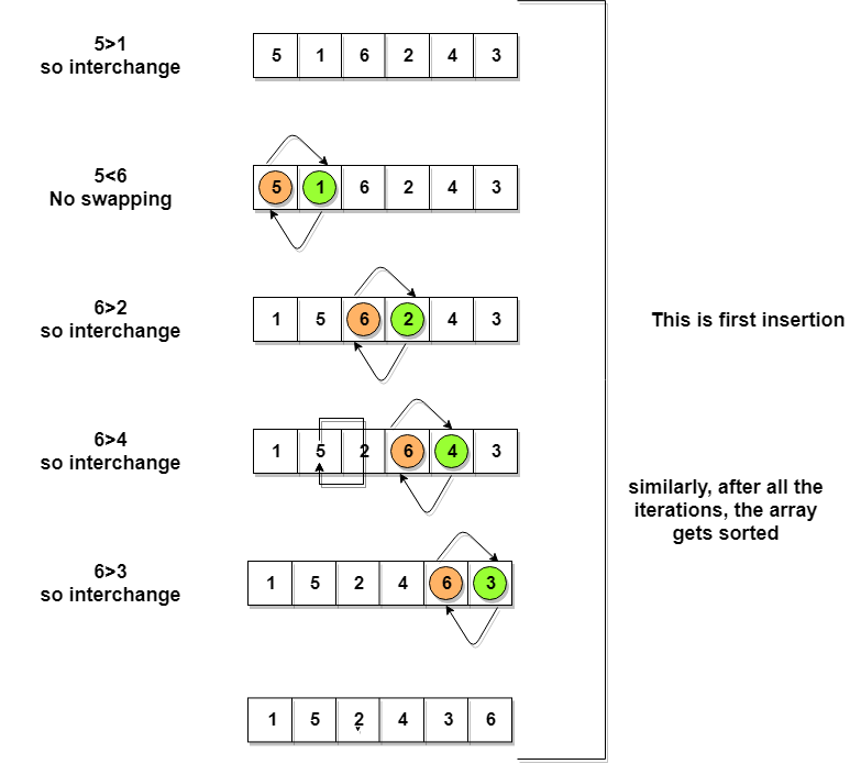
Let's consider an array with values
{5, 1, 6, 2, 4, 3}Below, we have a pictorial representation of how bubble sort will sort the given array.
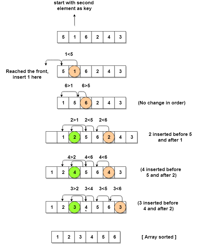
As you can see in the diagram above, after picking a
key, we start iterating over the elements to the left of thekey.We continue to move towards left if the elements are greater than the
keyelement and stop when we find the element which is less than thekeyelement.And, insert the
keyelement after the element which is less than thekeyelement.Implementing Insertion Sort Algorithm
Below we have a simple implementation of Insertion sort in C++ language.
#include <stdlib.h>
#include <iostream>

using namespace std;

//member functions declaration
void insertionSort(int arr[], int length);
void printArray(int array[], int size);

// main function
int main()
{
	int array[5] = {5, 1, 6, 2, 4, 3};
	// calling insertion sort function to sort the array
	insertionSort(array, 6);
	return 0;
}

void insertionSort(int arr[], int length)
{
	int i, j, key;
	for (i = 1; i < length; i++)
	{
		j = i;
 		while (j > 0 && arr[j - 1] > arr[j])
 		{
 			key = arr[j];
 			arr[j] = arr[j - 1];
 			arr[j - 1] = key;
 			j--;
 		}
	}
	cout << "Sorted Array: ";
	// print the sorted array
	printArray(arr, length);
}

// function to print the given array
void printArray(int array[], int size)
{
 	int j;
	for (j = 0; j < size; j++)
	{
 		cout <<" "<< array[j];
 	}
 	cout << endl;
}
Sorted Array: 1 2 3 4 5 6
Now let's try to understand the above simple insertion sort algorithm.
We took an array with 6 integers. We took a variable
key, in which we put each element of the array, during each pass, starting from the second element, that isa[1].Then using the
whileloop, we iterate, untiljbecomes equal to zero or we find an element which is greater thankey, and then we insert thekeyat that position.We keep on doing this, until
jbecomes equal to zero, or we encounter an element which is smaller than thekey, and then we stop. The currentkeyis now at the right position.We then make the next element as
keyand then repeat the same process.In the above array, first we pick 1 as
key, we compare it with 5(element before 1), 1 is smaller than 5, we insert 1 before 5. Then we pick 6 askey, and compare it with 5 and 1, no shifting in position this time. Then 2 becomes thekeyand is compared with 6 and 5, and then 2 is inserted after 1. And this goes on until the complete array gets sorted.Complexity Analysis of Insertion Sort
As we mentioned above that insertion sort is an efficient sorting algorithm, as it does not run on preset conditions using
forloops, but instead it uses onewhileloop, which avoids extra steps once the array gets sorted.Even though insertion sort is efficient, still, if we provide an already sorted array to the insertion sort algorithm, it will still execute the outer
forloop, thereby requiringnsteps to sort an already sorted array ofnelements, which makes its best case time complexity a linear function ofn.Worst Case Time Complexity [ Big-O ]: O(n2)
Best Case Time Complexity [Big-omega]: O(n)
Average Time Complexity [Big-theta]: O(n2)
Space Complexity: O(1)
Merge Sort Algorithm
Merge Sort follows the rule of Divide and Conquer to sort a given set of numbers/elements, recursively, hence consuming less time.
In the last two tutorials, we learned about Selection Sort and Insertion Sort, both of which have a worst-case running time of
O(n2). As the size of input grows, insertion and selection sort can take a long time to run.Merge sort , on the other hand, runs in
O(n*log n)time in all the cases.Before jumping on to, how merge sort works and it's implementation, first lets understand what is the rule of Divide and Conquer?
Divide and Conquer
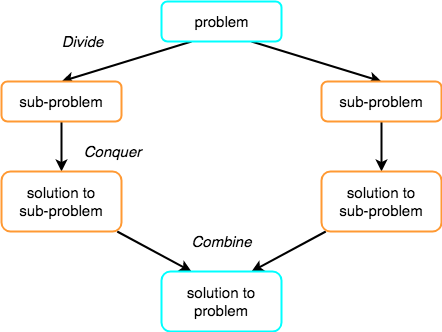
If we can break a single big problem into smaller sub-problems, solve the smaller sub-problems and combine their solutions to find the solution for the original big problem, it becomes easier to solve the whole problem.
Let's take an example, Divide and Rule.
When Britishers came to India, they saw a country with different religions living in harmony, hard working but naive citizens, unity in diversity, and found it difficult to establish their empire. So, they adopted the policy of Divide and Rule. Where the population of India was collectively a one big problem for them, they divided the problem into smaller problems, by instigating rivalries between local kings, making them stand against each other, and this worked very well for them.
Well that was history, and a socio-political policy (Divide and Rule), but the idea here is, if we can somehow divide a problem into smaller sub-problems, it becomes easier to eventually solve the whole problem.
In Merge Sort, the given unsorted array with
nelements, is divided intonsubarrays, each having one element, because a single element is always sorted in itself. Then, it repeatedly merges these subarrays, to produce new sorted subarrays, and in the end, one complete sorted array is produced.The concept of Divide and Conquer involves three steps:
- Divide the problem into multiple small problems.
- Conquer the subproblems by solving them. The idea is to break down the problem into atomic subproblems, where they are actually solved.
- Combine the solutions of the subproblems to find the solution of the actual problem.
How Merge Sort Works?
As we have already discussed that merge sort utilizes divide-and-conquer rule to break the problem into sub-problems, the problem in this case being, sorting a given array.
In merge sort, we break the given array midway, for example if the original array had
6elements, then merge sort will break it down into two subarrays with3elements each.But breaking the orignal array into 2 smaller subarrays is not helping us in sorting the array.
So we will break these subarrays into even smaller subarrays, until we have multiple subarrays with single element in them. Now, the idea here is that an array with a single element is already sorted, so once we break the original array into subarrays which has only a single element, we have successfully broken down our problem into base problems.
And then we have to merge all these sorted subarrays, step by step to form one single sorted array.
Let's consider an array with values
{14, 7, 3, 12, 9, 11, 6, 12}Below, we have a pictorial representation of how merge sort will sort the given array.
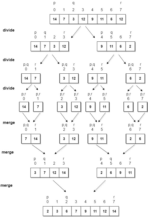
In merge sort we follow the following steps:
- We take a variable
pand store the starting index of our array in this. And we take another variablerand store the last index of array in it. - Then we find the middle of the array using the formula
(p + r)/2and mark the middle index asq, and break the array into two subarrays, fromptoqand fromq + 1torindex. - Then we divide these 2 subarrays again, just like we divided our main array and this continues.
- Once we have divided the main array into subarrays with single elements, then we start merging the subarrays.
Implementing Merge Sort Algorithm
Below we have a C program implementing merge sort algorithm.
/*
    a[] is the array, p is starting index, that is 0,
    and r is the last index of array.
*/

#include <stdio.h>

// lets take a[5] = {32, 45, 67, 2, 7} as the array to be sorted.

// merge sort function
void mergeSort(int a[], int p, int r)
{
    int q;
    if(p < r)
    {
        q = (p + r) / 2;
        mergeSort(a, p, q);
        mergeSort(a, q+1, r);
        merge(a, p, q, r);
    }
}

// function to merge the subarrays
void merge(int a[], int p, int q, int r)
{
    int b[5];   //same size of a[]
    int i, j, k;
    k = 0;
    i = p;
    j = q + 1;
    while(i <= q && j <= r)
    {
        if(a[i] < a[j])
        {
            b[k++] = a[i++];    // same as b[k]=a[i]; k++; i++;
        }
        else
        {
            b[k++] = a[j++];
        }
    }

    while(i <= q)
    {
        b[k++] = a[i++];
    }

    while(j <= r)
    {
        b[k++] = a[j++];
    }

    for(i=r; i >= p; i--)
    {
        a[i] = b[--k];  // copying back the sorted list to a[]
    }
}

// function to print the array
void printArray(int a[], int size)
{
    int i;
    for (i=0; i < size; i++)
    {
        printf("%d ", a[i]);
    }
    printf("\n");
}

int main()
{
    int arr[] = {32, 45, 67, 2, 7};
    int len = sizeof(arr)/sizeof(arr[0]);

    printf("Given array: \n");
    printArray(arr, len);

    // calling merge sort
    mergeSort(arr, 0, len - 1);

    printf("\nSorted array: \n");
    printArray(arr, len);
    return 0;
}
Given array: 32 45 67 2 7 Sorted array: 2 7 32 45 67
Complexity Analysis of Merge Sort
Merge Sort is quite fast, and has a time complexity of
O(n*log n). It is also a stable sort, which means the "equal" elements are ordered in the same order in the sorted list.In this section we will understand why the running time for merge sort is
O(n*log n).As we have already learned in Binary Search that whenever we divide a number into half in every stpe, it can be represented using a logarithmic function, which is
log nand the number of steps can be represented bylog n + 1(at most)Also, we perform a single step operation to find out the middle of any subarray, i.e.
O(1).And to merge the subarrays, made by dividing the original array of
nelements, a running time ofO(n)will be required.Hence the total time for
mergeSortfunction will becomen(log n + 1), which gives us a time complexity ofO(n*log n).Worst Case Time Complexity [ Big-O ]: O(n*log n)
Best Case Time Complexity [Big-omega]: O(n*log n)
Average Time Complexity [Big-theta]: O(n*log n)
Space Complexity: O(n)
- Time complexity of Merge Sort is
O(n*Log n)in all the 3 cases (worst, average and best) as merge sort always divides the array in two halves and takes linear time to merge two halves. - It requires equal amount of additional space as the unsorted array. Hence its not at all recommended for searching large unsorted arrays.
- It is the best Sorting technique used for sorting Linked Lists.
Quick Sort Algorithm
Quick Sort is also based on the concept of Divide and Conquer, just like merge sort. But in quick sort all the heavy lifting(major work) is done while dividing the array into subarrays, while in case of merge sort, all the real work happens during merging the subarrays. In case of quick sort, the combine step does absolutely nothing.
It is also called partition-exchange sort. This algorithm divides the list into three main parts:
- Elements less than the Pivot element
- Pivot element(Central element)
- Elements greater than the pivot element
Pivot element can be any element from the array, it can be the first element, the last element or any random element. In this tutorial, we will take the rightmost element or the last element as pivot.
For example: In the array
{52, 37, 63, 14, 17, 8, 6, 25}, we take25as pivot. So after the first pass, the list will be changed like this.{
6 8 17 142563 37 52}Hence after the first pass, pivot will be set at its position, with all the elements smaller to it on its left and all the elements larger than to its right. Now
6 8 17 14and63 37 52are considered as two separate sunarrays, and same recursive logic will be applied on them, and we will keep doing this until the complete array is sorted.How Quick Sorting Works?
Following are the steps involved in quick sort algorithm:
- After selecting an element as pivot, which is the last index of the array in our case, we divide the array for the first time.
- In quick sort, we call this partitioning. It is not simple breaking down of array into 2 subarrays, but in case of partitioning, the array elements are so positioned that all the elements smaller than the pivot will be on the left side of the pivot and all the elements greater than the pivot will be on the right side of it.
- And the pivot element will be at its final sorted position.
- The elements to the left and right, may not be sorted.
- Then we pick subarrays, elements on the left of pivot and elements on the right of pivot, and we perform partitioning on them by choosing a pivot in the subarrays.
Let's consider an array with values
{9, 7, 5, 11, 12, 2, 14, 3, 10, 6}Below, we have a pictorial representation of how quick sort will sort the given array.
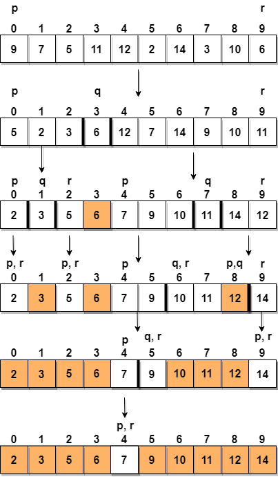
In step 1, we select the last element as the pivot, which is
6in this case, and call forpartitioning, hence re-arranging the array in such a way that6will be placed in its final position and to its left will be all the elements less than it and to its right, we will have all the elements greater than it.Then we pick the subarray on the left and the subarray on the right and select a pivot for them, in the above diagram, we chose
3as pivot for the left subarray and11as pivot for the right subarray.And we again call for
partitioning.Implementing Quick Sort Algorithm
Below we have a simple C program implementing the Quick sort algorithm:
// simple C program for Quick Sort
#include <stdio.h>
int partition(int a[], int beg, int end);
void quickSort(int a[], int beg, int end);
void main()
{
    int i;
    int arr[10]={90,23,101,45,65,28,67,89,34,29};
    quickSort(arr, 0, 9);
    printf("\n The sorted array is: \n");
    for(i=0;i<10;i++)
    printf(" %d\t", arr[i]);
}
int partition(int a[], int beg, int end)
{
    int left, right, temp, loc, flag;
    loc = left = beg;
    right = end;
    flag = 0;
    while(flag != 1)
    {
        while((a[loc] <= a[right]) && (loc!=right))
        right--;
        if(loc==right)
        flag =1;
        else if(a[loc]>a[right])
        {
            temp = a[loc];
            a[loc] = a[right];
            a[right] = temp;
            loc = right;
        }
        if(flag!=1)
        {
            while((a[loc] >= a[left]) && (loc!=left))
            left++;
            if(loc==left)
            flag =1;
            else if(a[loc] < a[left])
            {
                temp = a[loc];
                a[loc] = a[left];
                a[left] = temp;
                loc = left;
            }
        }
    }
    return loc;
}
void quickSort(int a[], int beg, int end)
{
    int loc;
    if(beg<end)
    {
        loc = partition(a, beg, end);
        quickSort(a, beg, loc-1);
        quickSort(a, loc+1, end);
    }
}
Complexity Analysis of Quick Sort
For an array, in which partitioning leads to unbalanced subarrays, to an extent where on the left side there are no elements, with all the elements greater than the pivot, hence on the right side.
And if keep on getting unbalanced subarrays, then the running time is the worst case, which is
O(n2)Where as if partitioning leads to almost equal subarrays, then the running time is the best, with time complexity as O(n*log n).
Worst Case Time Complexity [ Big-O ]: O(n2)
Best Case Time Complexity [Big-omega]: O(n*log n)
Average Time Complexity [Big-theta]: O(n*log n)
Space Complexity: O(n*log n)
As we know now, that if subarrays partitioning produced after partitioning are unbalanced, quick sort will take more time to finish. If someone knows that you pick the last index as pivot all the time, they can intentionally provide you with array which will result in worst-case running time for quick sort.
To avoid this, you can pick random pivot element too. It won't make any difference in the algorithm, as all you need to do is, pick a random element from the array, swap it with element at the last index, make it the pivot and carry on with quick sort.
- Space required by quick sort is very less, only
O(n*log n)additional space is required. - Quick sort is not a stable sorting technique, so it might change the occurence of two similar elements in the list while sorting.
Heap Sort Algorithm
Heap Sort is one of the best sorting methods being in-place and with no quadratic worst-case running time. Heap sort involves building a Heap data structure from the given array and then utilizing the Heap to sort the array.
You must be wondering, how converting an array of numbers into a heap data structure will help in sorting the array. To understand this, let's start by understanding what is a Heap.
What is a Heap ?
Heap is a special tree-based data structure, that satisfies the following special heap properties:
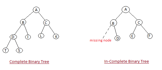
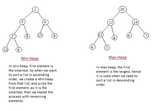
- Shape Property: Heap data structure is always a Complete Binary Tree, which means all levels of the tree are fully filled.
- Heap Property: All nodes are either greater than or equal to or less than or equal to each of its children. If the parent nodes are greater than their child nodes, heap is called a Max-Heap, and if the parent nodes are smaller than their child nodes, heap is called Min-Heap.
How Heap Sort Works?
Heap sort algorithm is divided into two basic parts:
- Creating a Heap of the unsorted list/array.
- Then a sorted array is created by repeatedly removing the largest/smallest element from the heap, and inserting it into the array. The heap is reconstructed after each removal.
Initially on receiving an unsorted list, the first step in heap sort is to create a Heap data structure(Max-Heap or Min-Heap). Once heap is built, the first element of the Heap is either largest or smallest(depending upon Max-Heap or Min-Heap), so we put the first element of the heap in our array. Then we again make heap using the remaining elements, to again pick the first element of the heap and put it into the array. We keep on doing the same repeatedly untill we have the complete sorted list in our array.
In the below algorithm, initially
heapsort()function is called, which callsheapify()to build the heap.Implementing Heap Sort Algorithm
Below we have a simple C++ program implementing the Heap sort algorithm.
/*  Below program is written in C++ language  */

#include <iostream>

using namespace std;

void heapify(int arr[], int n, int i)
{
    int largest = i;
    int l = 2*i + 1;
    int r = 2*i + 2;

    // if left child is larger than root
    if (l < n && arr[l] > arr[largest])
        largest = l;

    // if right child is larger than largest so far
    if (r < n && arr[r] > arr[largest])
        largest = r;

    // if largest is not root
    if (largest != i)
    {
        swap(arr[i], arr[largest]);

        // recursively heapify the affected sub-tree
        heapify(arr, n, largest);
    }
}

void heapSort(int arr[], int n)
{
    // build heap (rearrange array)
    for (int i = n / 2 - 1; i >= 0; i--)
        heapify(arr, n, i);

    // one by one extract an element from heap
    for (int i=n-1; i>=0; i--)
    {
        // move current root to end
        swap(arr[0], arr[i]);

        // call max heapify on the reduced heap
        heapify(arr, i, 0);
    }
}

/* function to print array of size n */
void printArray(int arr[], int n)
{
    for (int i = 0; i < n; i++)
    {
        cout << arr[i] << " ";
    }
    cout << "\n";
}


int main()
{
    int arr[] = {121, 10, 130, 57, 36, 17};
    int n = sizeof(arr)/sizeof(arr[0]);

    heapSort(arr, n);

    cout << "Sorted array is \n";
    printArray(arr, n);
}
Complexity Analysis of Heap Sort
Worst Case Time Complexity: O(n*log n)
Best Case Time Complexity: O(n*log n)
Average Time Complexity: O(n*log n)
Space Complexity : O(1)
- Heap sort is not a Stable sort, and requires a constant space for sorting a list.
- Heap Sort is very fast and is widely used for sorting.
- Shape Property: Heap data structure is always a Complete Binary Tree, which means all levels of the tree are fully filled.
Counting Sort Algorithm
Counting Sort Algorithm is an efficient sorting algorithm that can be used for sorting elements within a specific range. This sorting technique is based on the frequency/count of each element to be sorted and works using the following algorithm-
- Input: Unsorted array A[] of n elements
- Output: Sorted arrayB[]
Step 1: Consider an input array A having n elements in the range of 0 to k, where n and k are positive integer numbers. These n elements have to be sorted in ascending order using the counting sort technique. Also note that A[] can have distinct or duplicate elements
Step 2: The count/frequency of each distinct element in A is computed and stored in another array, say count, of size k+1. Let u be an element in A such that its frequency is stored at count[u].
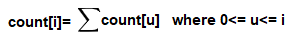
Step 3: Update the count array so that element at each index, say i, is equal to -
Step 4: The updated count array gives the index of each element of array A in the sorted sequence. Assume that the sorted sequence is stored in an output array, say B, of size n.
Step 5: Add each element from input array A to B as follows:
- Set i=0 and
t = A[i] - Add t to B[v] such that
v = (count[t]-1). - Decrement count[t] by 1
- Increment i by 1
Repeat steps (a) to (d) till i = n-1
Step 6: Display B since this is the sorted array
Pictorial Representation of Counting Sort with an Example
Let us trace the above algorithm using an example:
Consider the following input array A to be sorted. All the elements are in range 0 to 9
A[]= {1, 3, 2, 8, 5, 1, 5, 1, 2, 7}Step 1: Initialize an auxiliary array, say count and store the frequency of every distinct element. Size of count is 10 (k+1, such that range of elements in A is 0 to k)
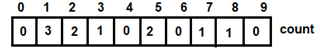 Figure 1: count array
Step 2: Using the formula, updated count array is -
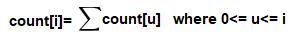 Figure 2: Formula for updating count array
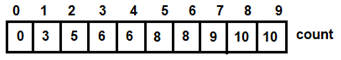 Figure 3 : Updated count array
Step 3: Add elements of array A to resultant array B using the following steps:
- For, i=0, t=1, count[1]=3, v=2. After adding 1 to B[2], count[1]=2 and i=1
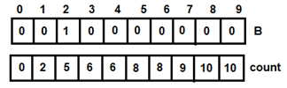 Figure 4: For i=0
 - For i=1, t=3, count[3]=6, v=5. After adding 3 to B[5], count[3]=5 and i=2
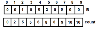 Figure 5: For i=1
 - For i=2, t=2, count[2]= 5, v=4. After adding 2 to B[4], count[2]=4 and i=3
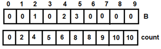 Figure 6: For i=2
 - For i=3, t=8, count[8]= 10, v=9. After adding 8 to B[9], count[8]=9 and i=4
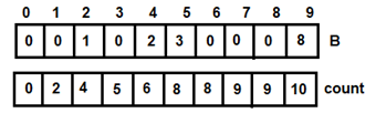 Figure 7: For i=3
 - On similar lines, we have the following:
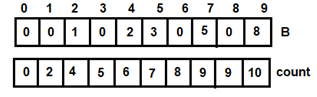 Figure 8: For i=4
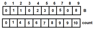 Figure 9: For i=5
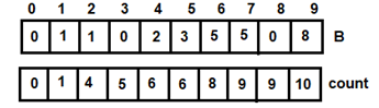 Figure 10: For i=6
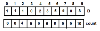 Figure 11: For i=7
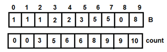 Figure 12: For i=8
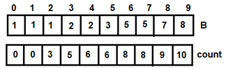 Figure 13: For i=9
Thus, array
Bhas the sorted list of elements.Program for Counting Sort Algorithm
Below we have a simple program in C++ implementing the counting sort algorithm:
#include<iostream>
using namespace std;

int k=0; 	// for storing the maximum element of input array

/* Method to sort the array */
void sort_func(int A[],int B[],int n)
{
	int count[k+1],t;
	for(int i=0;i<=k;i++)
	{
		//Initialize array count
		count[i] = 0;
	}
	for(int i=0;i<n;i++)
	{
	    // count the occurrence of elements u of A
	    // & increment count[u] where u=A[i]
		t = A[i];
		count[t]++;
	}
	for(int i=1;i<=k;i++)
	{
	    // Updating elements of count array
		count[i] = count[i]+count[i-1];
	}
	for(int i=0;i<n;i++)
	{
		// Add elements of array A to array B
		t = A[i];
		B[count[t]] = t;
	    // Decrement the count value by 1
		count[t]=count[t]-1;
	}
}
int main()
{
	int n;
	cout<<"Enter the size of the array :";
	cin>>n;

	// A is the input array and will store elements entered by the user
	// B is the output array having the sorted elements
	int A[n],B[n];
	cout<<"Enter the array elements: ";
	for(int i=0;i<n;i++)
	{
		cin>>A[i];
		if(A[i]>k)
		{
			// k will have the maximum element of A[]
			k = A[i];
		}
	}

	sort_func(A,B,n);

	// Printing the elements of array B
	for(int i=1;i<=n;i++)
	{
		cout<<B[i]<<" ";
	}

	cout<<"\n";
	return 0;
}
The input array is the same as that used in the example:
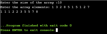 Figure 14: Output of Program
Note: The algorithm can be mapped to any programming language as per the requirement.
Time Complexity Analysis
For scanning the input array elements, the loop iterates n times, thus taking
O(n)running time. The sorted array B[] also gets computed in n iterations, thus requiring O(n) running time. The count array also uses k iterations, thus has a running time of O(k). Thus the total running time for counting sort algorithm isO(n+k).Key Points:
- The above implementation of Counting Sort can also be extended to sort negative input numbers
- Since counting sort is suitable for sorting numbers that belong to a well-defined, finite and small range, it can be used asa subprogram in other sorting algorithms like radix sort which can be used for sorting numbers having a large range
- Counting Sort algorithm is efficient if the range of input data (k) is not much greater than the number of elements in the input array (n). It will not work if we have 5 elements to sort in the range of 0 to 10,000
- It is an integer-based sorting algorithm unlike others which are usually comparison-based. A comparison-based sorting algorithm sorts numbers only by comparing pairs of numbers. Few examples of comparison based sorting algorithms are quick sort, merge sort, bubble sort, selection sort, heap sort, insertion sort, whereas algorithms like radix sort, bucket sort and comparison sort fall into the category of non-comparison based sorting algorithms.
Advantages of Counting Sort:
- It is quite fast
- It is a stable algorithm
Note: For a sorting algorithm to be stable, the order of elements with equal keys (values) in the sorted array should be the same as that of the input array.
Disadvantages of Counting Sort:
- It is not suitable for sorting large data sets
- It is not suitable for sorting string values
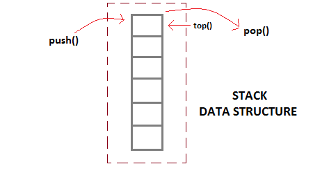
What is Stack Data Structure?
Stack is an abstract data type with a bounded(predefined) capacity. It is a simple data structure that allows adding and removing elements in a particular order. Every time an element is added, it goes on the top of the stack and the only element that can be removed is the element that is at the top of the stack, just like a pile of objects.
Basic features of Stack
- Stack is an ordered list of similar data type.
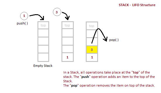
- Stack is a LIFO(Last in First out) structure or we can say FILO(First in Last out).
push()function is used to insert new elements into the Stack andpop()function is used to remove an element from the stack. Both insertion and removal are allowed at only one end of Stack called Top.- Stack is said to be in Overflow state when it is completely full and is said to be in Underflow state if it is completely empty.
Applications of Stack
The simplest application of a stack is to reverse a word. You push a given word to stack - letter by letter - and then pop letters from the stack.
There are other uses also like:
- Parsing
- Expression Conversion(Infix to Postfix, Postfix to Prefix etc)
Implementation of Stack Data Structure
Stack can be easily implemented using an Array or a Linked List. Arrays are quick, but are limited in size and Linked List requires overhead to allocate, link, unlink, and deallocate, but is not limited in size. Here we will implement Stack using array.
Algorithm for PUSH operation
- Check if the stack is full or not.
- If the stack is full, then print error of overflow and exit the program.
- If the stack is not full, then increment the top and add the element.
Algorithm for POP operation
- Check if the stack is empty or not.
- If the stack is empty, then print error of underflow and exit the program.
- If the stack is not empty, then print the element at the top and decrement the top.
Below we have a simple C++ program implementing stack data structure while following the object oriented programming concepts.
/*  Below program is written in C++ language  */

# include<iostream>

using namespace std;

class Stack
{
    int top;
    public:
    int a[10];  //Maximum size of Stack
    Stack()
    {
        top = -1;
    }

    // declaring all the function
    void push(int x);
    int pop();
    void isEmpty();
};

// function to insert data into stack
void Stack::push(int x)
{
    if(top >= 10)
    {
        cout << "Stack Overflow \n";
    }
    else
    {
        a[++top] = x;
        cout << "Element Inserted \n";
    }
}

// function to remove data from the top of the stack
int Stack::pop()
{
    if(top < 0)
    {
        cout << "Stack Underflow \n";
        return 0;
    }
    else
    {
        int d = a[top--];
        return d;
    }
}

// function to check if stack is empty
void Stack::isEmpty()
{
    if(top < 0)
    {
        cout << "Stack is empty \n";
    }
    else
    {
        cout << "Stack is not empty \n";
    }
}

// main function
int main() {

    Stack s1;
    s1.push(10);
    s1.push(100);
    /*
        preform whatever operation you want on the stack
    */
}
Position of TopStatus of Stack-1Stack is Empty 0Only one element in Stack N-1Stack is Full NOverflow state of Stack Analysis of Stack Operations
Below mentioned are the time complexities for various operations that can be performed on the Stack data structure.
- Push Operation : O(1)
- Pop Operation : O(1)
- Top Operation : O(1)
- Search Operation : O(n)
The time complexities for
push()andpop()functions areO(1)because we always have to insert or remove the data from the top of the stack, which is a one step process.- Like stack, queue is also an ordered list of elements of similar data types.
- Queue is a FIFO( First in First Out ) structure.
- Once a new element is inserted into the Queue, all the elements inserted before the new element in the queue must be removed, to remove the new element.
peek( )function is oftenly used to return the value of first element without dequeuing it.- Serving requests on a single shared resource, like a printer, CPU task scheduling etc.
- In real life scenario, Call Center phone systems uses Queues to hold people calling them in an order, until a service representative is free.
- Handling of interrupts in real-time systems. The interrupts are handled in the same order as they arrive i.e First come first served.
- Check if the queue is full or not.
- If the queue is full, then print overflow error and exit the program.
- If the queue is not full, then increment the tail and add the element.
- Check if the queue is empty or not.
- If the queue is empty, then print underflow error and exit the program.
- If the queue is not empty, then print the element at the head and increment the head.
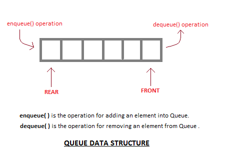
What is a Queue Data Structure?
Queue is also an abstract data type or a linear data structure, just like stack data structure, in which the first element is inserted from one end called the REAR(also called tail), and the removal of existing element takes place from the other end called as FRONT(also called head).
This makes queue as FIFO(First in First Out) data structure, which means that element inserted first will be removed first.
Which is exactly how queue system works in real world. If you go to a ticket counter to buy movie tickets, and are first in the queue, then you will be the first one to get the tickets. Right? Same is the case with Queue data structure. Data inserted first, will leave the queue first.
The process to add an element into queue is called Enqueue and the process of removal of an element from queue is called Dequeue.
Basic features of Queue
Applications of Queue
Queue, as the name suggests is used whenever we need to manage any group of objects in an order in which the first one coming in, also gets out first while the others wait for their turn, like in the following scenarios:
Implementation of Queue Data Structure
Queue can be implemented using an Array, Stack or Linked List. The easiest way of implementing a queue is by using an Array.
Initially the head(FRONT) and the tail(REAR) of the queue points at the first index of the array (starting the index of array from 0). As we add elements to the queue, the tail keeps on moving ahead, always pointing to the position where the next element will be inserted, while the head remains at the first index.
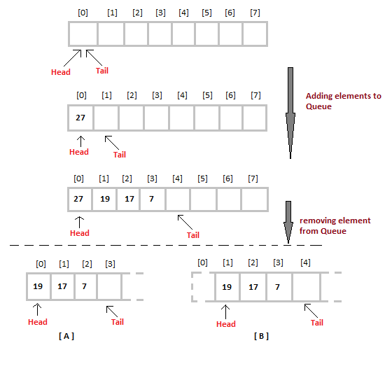
When we remove an element from Queue, we can follow two possible approaches (mentioned [A] and [B] in above diagram). In [A] approach, we remove the element at head position, and then one by one shift all the other elements in forward position.
In approach [B] we remove the element from head position and then move head to the next position.
In approach [A] there is an overhead of shifting the elements one position forward every time we remove the first element.
In approach [B] there is no such overhead, but whenever we move head one position ahead, after removal of first element, the size on Queue is reduced by one space each time.
Algorithm for ENQUEUE operation
Algorithm for DEQUEUE operation
/* Below program is written in C++ language */

#include<iostream>

using namespace std;

#define SIZE 10

class Queue
{
    int a[SIZE];
    int rear;   //same as tail
    int front;  //same as head

    public:
    Queue()
    {
        rear = front = -1;
    }

    //declaring enqueue, dequeue and display functions
    void enqueue(int x);
    int dequeue();
    void display();
};

// function enqueue - to add data to queue
void Queue :: enqueue(int x)
{
    if(front == -1) {
        front++;
    }
    if( rear == SIZE-1)
    {
        cout << "Queue is full";
    }
    else
    {
        a[++rear] = x;
    }
}

// function dequeue - to remove data from queue
int Queue :: dequeue()
{
    return a[++front];  // following approach [B], explained above
}

// function to display the queue elements
void Queue :: display()
{
    int i;
    for( i = front; i <= rear; i++)
    {
        cout << a[i] << endl;
    }
}

// the main function
int main()
{
    Queue q;
    q.enqueue(10);
    q.enqueue(100);
    q.enqueue(1000);
    q.enqueue(1001);
    q.enqueue(1002);
    q.dequeue();
    q.enqueue(1003);
    q.dequeue();
    q.dequeue();
    q.enqueue(1004);

    q.display();

    return 0;
}
To implement approach [A], you simply need to change the dequeue method, and include a for loop which will shift all the remaining elements by one position.
return a[0];    //returning first element
for (i = 0; i < tail-1; i++)    //shifting all other elements
{
    a[i] = a[i+1];
    tail--;
}
Complexity Analysis of Queue Operations
Just like Stack, in case of a Queue too, we know exactly, on which position new element will be added and from where an element will be removed, hence both these operations requires a single step.
- Enqueue: O(1)
- Dequeue: O(1)
- Size: O(1)
What is a Circular Queue?
Before we start to learn about Circular queue, we should first understand, why we need a circular queue, when we already have linear queue data structure.
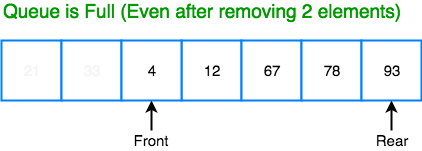
In a Linear queue, once the queue is completely full, it's not possible to insert more elements. Even if we dequeue the queue to remove some of the elements, until the queue is reset, no new elements can be inserted. You must be wondering why?
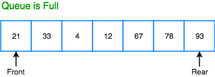
When we dequeue any element to remove it from the queue, we are actually moving the front of the queue forward, thereby reducing the overall size of the queue. And we cannot insert new elements, because the rear pointer is still at the end of the queue.
The only way is to reset the linear queue, for a fresh start.
Circular Queue is also a linear data structure, which follows the principle of FIFO(First In First Out), but instead of ending the queue at the last position, it again starts from the first position after the last, hence making the queue behave like a circular data structure.
Basic features of Circular Queue
- In case of a circular queue,
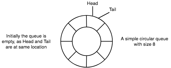
headpointer will always point to the front of the queue, andtailpointer will always point to the end of the queue. - Initially, the head and the tail pointers will be pointing to the same location, this would mean that the queue is empty.
- New data is always added to the location pointed by the
tailpointer, and once the data is added,tailpointer is incremented to point to the next available location.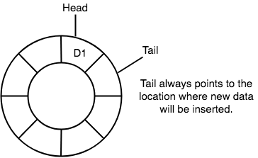
- In a circular queue, data is not actually removed from the queue. Only the
headpointer is incremented by one position when dequeue is executed. As the queue data is only the data betweenheadandtail, hence the data left outside is not a part of the queue anymore, hence removed.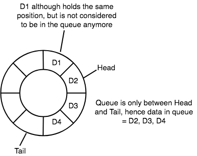
- The
headand thetailpointer will get reinitialised to 0 every time they reach the end of the queue.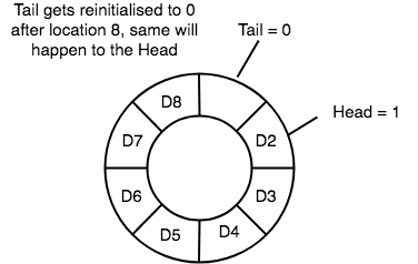
- Also, the
headand thetailpointers can cross each other. In other words,headpointer can be greater than thetail. Sounds odd? This will happen when we dequeue the queue a couple of times and thetailpointer gets reinitialised upon reaching the end of the queue.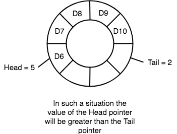
Going Round and Round
Another very important point is keeping the value of the tail and the head pointer within the maximum queue size.
In the diagrams above the queue has a size of 8, hence, the value of tail and head pointers will always be between 0 and 7.
This can be controlled either by checking everytime whether tail or head have reached the maxSize and then setting the value 0 or, we have a better way, which is, for a value x if we divide it by 8, the remainder will never be greater than 8, it will always be between 0 and 0, which is exactly what we want.
So the formula to increment the head and tail pointers to make them go round and round over and again will be, head = (head+1) % maxSize or tail = (tail+1) % maxSize
Application of Circular Queue
Below we have some common real-world examples where circular queues are used:
- Computer controlled Traffic Signal System uses circular queue.
- CPU scheduling and Memory management.
Implementation of Circular Queue
Below we have the implementation of a circular queue:
- Initialize the queue, with size of the queue defined (
maxSize), andheadandtailpointers. enqueue: Check if the number of elements is equal to maxSize - 1:- If Yes, then return Queue is full.
- If No, then add the new data element to the location of
tailpointer and increment thetailpointer.
dequeue: Check if the number of elements in the queue is zero:- If Yes, then return Queue is empty.
- If No, then increment the
headpointer.
- Finding the
size:- If, tail >= head,
size = (tail - head) + 1 - But if, head > tail, then
size = maxSize - (head - tail) + 1
- If, tail >= head,
/* Below program is written in C++ language */

#include<iostream>

using namespace std;

#define SIZE 10

class CircularQueue
{
    int a[SIZE];
    int rear;   //same as tail
    int front;  //same as head

    public:
    CircularQueue()
    {
        rear = front = -1;
    }

    // function to check if queue is full
    bool isFull()
    {
        if(front == 0 && rear == SIZE - 1)
        {
            return true;
        }
        if(front == rear + 1)
        {
            return true;
        }
        return false;
    }

    // function to check if queue is empty
    bool isEmpty()
    {
        if(front == -1)
        {
            return true;
        }
        else
        {
            return false;
        }
    }

    //declaring enqueue, dequeue, display and size functions
    void enqueue(int x);
    int dequeue();
    void display();
    int size();
};

// function enqueue - to add data to queue
void CircularQueue :: enqueue(int x)
{
    if(isFull())
    {
        cout << "Queue is full";
    }
    else
    {
        if(front == -1)
        {
            front = 0;
        }
        rear = (rear + 1) % SIZE;   // going round and round concept
        // inserting the element
        a[rear] = x;
        cout << endl << "Inserted " << x << endl;
    }
}

// function dequeue - to remove data from queue
int CircularQueue :: dequeue()
{
    int y;

    if(isEmpty())
    {
        cout << "Queue is empty" << endl;
    }
    else
    {
        y = a[front];
        if(front == rear)
        {
            // only one element in queue, reset queue after removal
            front = -1;
            rear = -1;
        }
        else
        {
            front = (front+1) % SIZE;
        }
        return(y);
    }
}

void CircularQueue :: display()
{
    /* Function to display status of Circular Queue */
    int i;
    if(isEmpty())
    {
        cout << endl << "Empty Queue" << endl;
    }
    else
    {
        cout << endl << "Front -> " << front;
        cout << endl << "Elements -> ";
        for(i = front; i != rear; i= (i+1) % SIZE)
        {
            cout << a[i] << "\t";
        }
        cout << a[i];
        cout << endl << "Rear -> " << rear;
    }
}

int CircularQueue :: size()
{
    if(rear >= front)
    {
        return (rear - front) + 1;
    }
    else
    {
        return (SIZE - (front - rear) + 1);
    }
}

// the main function
int main()
{
    CircularQueue cq;
    cq.enqueue(10);
    cq.enqueue(100);
    cq.enqueue(1000);

    cout << endl << "Size of queue: " << cq.size();

    cout << endl << "Removed element: " << cq.dequeue();

    cq.display();

    return 0;
}
Inserted 10 Inserted 100 Inserted 1000 Size of queue: 3 Removed element: 10 Front -> 1 Elements -> 100 1000 Rear -> 2
What is a Circular Queue?
Before we start to learn about Circular queue, we should first understand, why Uwe need a circular queue, when we already have linear queue data structure.
In a Linear queue, once the queue is completely full, it's not possible to insert more elements. Even if we dequeue the queue to remove some of the elements, until the queue is reset, no new elements can be inserted. You must be wondering why?
When we dequeue any element to remove it from the queue, we are actually moving the front of the queue forward, thereby reducing the overall size of the queue. And we cannot insert new elements, because the rear pointer is still at the end of the queue.
The only way is to reset the linear queue, for a fresh start.
Circular Queue is also a linear data structure, which follows the principle of FIFO(First In First Out), but instead of ending the queue at the last position, it again starts from the first position after the last, hence making the queue behave like a circular data structure.
Basic features of Circular Queue
- In case of a circular queue,
headpointer will always point to the front of the queue, andtailpointer will always point to the end of the queue. - Initially, the head and the tail pointers will be pointing to the same location, this would mean that the queue is empty.
- New data is always added to the location pointed by the
tailpointer, and once the data is added,tailpointer is incremented to point to the next available location. - In a circular queue, data is not actually removed from the queue. Only the
headpointer is incremented by one position when dequeue is executed. As the queue data is only the data betweenheadandtail, hence the data left outside is not a part of the queue anymore, hence removed. - The
headand thetailpointer will get reinitialised to 0 every time they reach the end of the queue. - Also, the
headand thetailpointers can cross each other. In other words,headpointer can be greater than thetail. Sounds odd? This will happen when we dequeue the queue a couple of times and thetailpointer gets reinitialised upon reaching the end of the queue.
Going Round and Round
Another very important point is keeping the value of the tail and the head pointer within the maximum queue size.
In the diagrams above the queue has a size of 8, hence, the value of tail and head pointers will always be between 0 and 7.
This can be controlled either by checking everytime whether tail or head have reached the maxSize and then setting the value 0 or, we have a better way, which is, for a value x if we divide it by 8, the remainder will never be greater than 8, it will always be between 0 and 0, which is exactly what we want.
So the formula to increment the head and tail pointers to make them go round and round over and again will be, head = (head+1) % maxSize or tail = (tail+1) % maxSize
Application of Circular Queue
Below we have some common real-world examples where circular queues are used:
- Computer controlled Traffic Signal System uses circular queue.
- CPU scheduling and Memory management.
Implementation of Circular Queue
Below we have the implementation of a circular queue:
- Initialize the queue, with size of the queue defined (
maxSize), andheadandtailpointers. enqueue: Check if the number of elements is equal to maxSize - 1:- If Yes, then return Queue is full.
- If No, then add the new data element to the location of
tailpointer and increment thetailpointer.
dequeue: Check if the number of elements in the queue is zero:- If Yes, then return Queue is empty.
- If No, then increment the
headpointer.
- Finding the
size:- If, tail >= head,
size = (tail - head) + 1 - But if, head > tail, then
size = maxSize - (head - tail) + 1
- If, tail >= head,
/* Below program is written in C++ language */

#include<iostream>

using namespace std;

#define SIZE 10

class CircularQueue
{
    int a[SIZE];
    int rear;   //same as tail
    int front;  //same as head

    public:
    CircularQueue()
    {
        rear = front = -1;
    }

    // function to check if queue is full
    bool isFull()
    {
        if(front == 0 && rear == SIZE - 1)
        {
            return true;
        }
        if(front == rear + 1)
        {
            return true;
        }
        return false;
    }

    // function to check if queue is empty
    bool isEmpty()
    {
        if(front == -1)
        {
            return true;
        }
        else
        {
            return false;
        }
    }

    //declaring enqueue, dequeue, display and size functions
    void enqueue(int x);
    int dequeue();
    void display();
    int size();
};

// function enqueue - to add data to queue
void CircularQueue :: enqueue(int x)
{
    if(isFull())
    {
        cout << "Queue is full";
    }
    else
    {
        if(front == -1)
        {
            front = 0;
        }
        rear = (rear + 1) % SIZE;   // going round and round concept
        // inserting the element
        a[rear] = x;
        cout << endl << "Inserted " << x << endl;
    }
}

// function dequeue - to remove data from queue
int CircularQueue :: dequeue()
{
    int y;

    if(isEmpty())
    {
        cout << "Queue is empty" << endl;
    }
    else
    {
        y = a[front];
        if(front == rear)
        {
            // only one element in queue, reset queue after removal
            front = -1;
            rear = -1;
        }
        else
        {
            front = (front+1) % SIZE;
        }
        return(y);
    }
}

void CircularQueue :: display()
{
    /* Function to display status of Circular Queue */
    int i;
    if(isEmpty())
    {
        cout << endl << "Empty Queue" << endl;
    }
    else
    {
        cout << endl << "Front -> " << front;
        cout << endl << "Elements -> ";
        for(i = front; i != rear; i= (i+1) % SIZE)
        {
            cout << a[i] << "\t";
        }
        cout << a[i];
        cout << endl << "Rear -> " << rear;
    }
}

int CircularQueue :: size()
{
    if(rear >= front)
    {
        return (rear - front) + 1;
    }
    else
    {
        return (SIZE - (front - rear) + 1);
    }
}

// the main function
int main()
{
    CircularQueue cq;
    cq.enqueue(10);
    cq.enqueue(100);
    cq.enqueue(1000);

    cout << endl << "Size of queue: " << cq.size();

    cout << endl << "Removed element: " << cq.dequeue();

    cq.display();

    return 0;
}
Inserted 10 Inserted 100 Inserted 1000 Size of queue: 3 Removed element: 10 Front -> 1 Elements -> 100 1000 Rear -> 2
Introduction to Linked Lists
Linked List is a very commonly used linear data structure which consists of group of nodes in a sequence.
Each node holds its own data and the address of the next node hence forming a chain like structure.
Linked Lists are used to create trees and graphs.
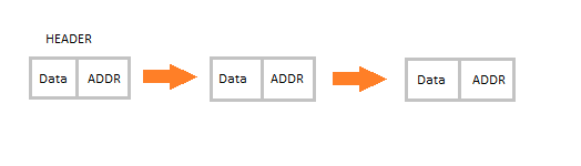
Advantages of Linked Lists
- They are a dynamic in nature which allocates the memory when required.
- Insertion and deletion operations can be easily implemented.
- Stacks and queues can be easily executed.
- Linked List reduces the access time.
Disadvantages of Linked Lists
- The memory is wasted as pointers require extra memory for storage.
- No element can be accessed randomly; it has to access each node sequentially.
- Reverse Traversing is difficult in linked list.
Applications of Linked Lists
- Linked lists are used to implement stacks, queues, graphs, etc.
- Linked lists let you insert elements at the beginning and end of the list.
- In Linked Lists we don't need to know the size in advance.
Types of Linked Lists
There are 3 different implementations of Linked List available, they are:
- Singly Linked List
- Doubly Linked List
- Circular Linked List
Let's know more about them and how they are different from each other.
Singly Linked List
Singly linked lists contain nodes which have a data part as well as an address part i.e. next, which points to the next node in the sequence of nodes.
The operations we can perform on singly linked lists are insertion, deletion and traversal.
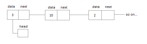
Doubly Linked List
In a doubly linked list, each node contains a data part and two addresses, one for the previous node and one for the next node.
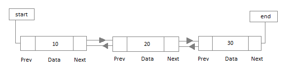
Circular Linked List
In circular linked list the last node of the list holds the address of the first node hence forming a circular chain.
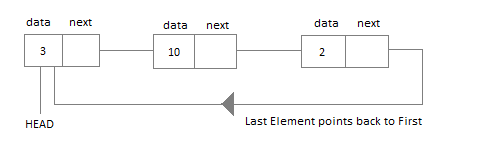
We will learn about all the 3 types of linked list, one by one, in the next tutorials. So click on Next button, let's learn more about linked lists.
Difference between Array and Linked List
Both Linked List and Array are used to store linear data of similar type, but an array consumes contiguous memory locations allocated at compile time, i.e. at the time of declaration of array, while for a linked list, memory is assigned as and when data is added to it, which means at runtime.
This is the basic and the most important difference between a linked list and an array. In the section below, we will discuss this in details along with highlighting other differences.
Linked List vs. Array
Array is a datatype which is widely implemented as a default type, in almost all the modern programming languages, and is used to store data of similar type.
But there are many usecases, like the one where we don't know the quantity of data to be stored, for which advanced data structures are required, and one such data structure is linked list.
Let's understand how array is different from Linked list.
| ARRAY | LINKED LIST |
|---|---|
| Array is a collection of elements of similar data type. | Linked List is an ordered collection of elements of same type, which are connected to each other using pointers. |
Array supports Random Access, which means elements can be accessed directly using their index, like Hence, accessing elements in an array is fast with a constant time complexity of | Linked List supports Sequential Access, which means to access any element/node in a linked list, we have to sequentially traverse the complete linked list, upto that element. To access nth element of a linked list, time complexity is |
In an array, elements are stored in contiguous memory location or consecutive manner in the memory. | In a linked list, new elements can be stored anywhere in the memory. Address of the memory location allocated to the new element is stored in the previous node of linked list, hence formaing a link between the two nodes/elements. |
| In array, Insertion and Deletion operation takes more time, as the memory locations are consecutive and fixed. | In case of linked list, a new element is stored at the first free and available memory location, with only a single overhead step of storing the address of memory location in the previous node of linked list. Insertion and Deletion operations are fast in linked list. |
| Memory is allocated as soon as the array is declared, at compile time. It's also known as Static Memory Allocation. | Memory is allocated at runtime, as and when a new node is added. It's also known as Dynamic Memory Allocation. |
| In array, each element is independent and can be accessed using it's index value. | In case of a linked list, each node/element points to the next, previous, or maybe both nodes. |
| Array can single dimensional, two dimensional or multidimensional | Linked list can be Linear(Singly), Doubly or Circular linked list. |
| Size of the array must be specified at time of array decalaration. | Size of a Linked list is variable. It grows at runtime, as more nodes are added to it. |
| Array gets memory allocated in the Stack section. | Whereas, linked list gets memory allocated in Heap section. |
Below we have a pictorial representation showing how consecutive memory locations are allocated for array, while in case of linked list random memory locations are assigned to nodes, but each node is connected to its next node using pointer.
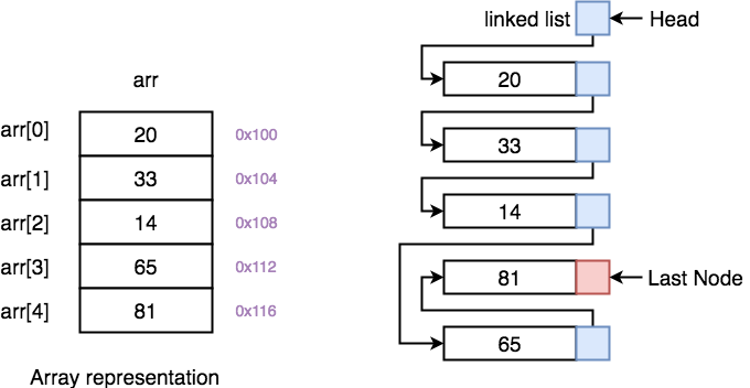
On the left, we have Array and on the right, we have Linked List.
Why we need pointers in Linked List? [Deep Dive]
In case of array, memory is allocated in contiguous manner, hence array elements get stored in consecutive memory locations. So when you have to access any array element, all we have to do is use the array index, for example arr[4] will directly access the 5th memory location, returning the data stored there.
But in case of linked list, data elements are allocated memory at runtime, hence the memory location can be anywhere. Therefore to be able to access every node of the linked list, address of every node is stored in the previous node, hence forming a link between every node.
We need this additional pointer because without it, the data stored at random memory locations will be lost. We need to store somewhere all the memory locations where elements are getting stored.
Yes, this requires an additional memory space with each node, which means an additional space of O(n) for every n node linked list.
Linear Linked List
Linear Linked list is the default linked list and a linear data structure in which data is not stored in contiguous memory locations but each data node is connected to the next data node via a pointer, hence forming a chain.
The element in such a linked list can be inserted in 2 ways:
- Insertion at beginning of the list.
- Insertion at the end of the list.
Hence while writing the code for Linked List we will include methods to insert or add new data elements to the linked list, both, at the beginning of the list and at the end of the list.
We will also be adding some other useful methods like:
- Checking whether Linked List is empty or not.
- Searching any data element in the Linked List
- Deleting a particular Node(data element) from the List
Before learning how we insert data and create a linked list, we must understand the components forming a linked list, and the main component is the Node.
What is a Node?
A Node in a linked list holds the data value and the pointer which points to the location of the next node in the linked list.
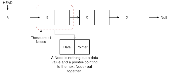
In the picture above we have a linked list, containing 4 nodes, each node has some data(A, B, C and D) and a pointer which stores the location of the next node.
You must be wondering why we need to store the location of the next node. Well, because the memory locations allocated to these nodes are not contiguous hence each node should know where the next node is stored.
As the node is a combination of multiple information, hence we will be defining a class for Node which will have a variable to store data and another variable to store the pointer. In C language, we create a structure using the struct keyword.
class Node
{
    public:
    // our linked list will only hold int data
    int data;
    //pointer to the next node
    node* next;

    // default constructor
    Node()
    {
        data = 0;
        next = NULL;
    }

    // parameterised constructor
    Node(int x)
    {
        data = x;
        next = NULL;
    }
}
We can also make the Node class properties data and next as private, in that case we will need to add the getter and setter methods to access them(don't know what getter and setter methods are: Inline Functions in C++ ). You can add the getter and setter functions to the Node class like this:
class Node
{
    // our linked list will only hold int data
    int data;
    //pointer to the next node
    node* next;

    // default constructor same as above

    // parameterised constructor same as above

    /* getters and setters */
    // get the value of data
    int getData()
    {
        return data;
    }

    // to set the value for data
    void setData(int x)
    {
        this.data = x;
    }
    // get the value of next pointer
    node* getNext()
    {
        return next;
    }
    // to set the value for pointer
    void setNext(node *n)
    {
        this.next = n;
    }
}
The Node class basically creates a node for the data to be included into the Linked List. Once the object for the class Node is created, we use various functions to fit in that node into the Linked List.
Linked List class
As we are following the complete OOPS methodology, hence we will create a separate class for Linked List, which will have all the methods like insertion, search, deletion etc. Also, the linked list class will have a pointer called head to store the location of the first node which will be added to the linked list.
class LinkedList
{
    public:
    node *head;
    //declaring the functions

    //function to add Node at front
    int addAtFront(node *n);
    //function to check whether Linked list is empty
    int isEmpty();
    //function to add Node at the End of list
    int addAtEnd(node *n);
    //function to search a value
    node* search(int k);
    //function to delete any Node
    node* deleteNode(int x);

    LinkedList()
    {
        head = NULL;
    }
}
Insertion at the Beginning
Steps to insert a Node at beginning :
- The first Node is the Head for any Linked List.
- When a new Linked List is instantiated, it just has the Head, which is Null.
- Else, the Head holds the pointer to the first Node of the List.
- When we want to add any Node at the front, we must make the head point to it.
- And the Next pointer of the newly added Node, must point to the previous Head, whether it be NULL(in case of new List) or the pointer to the first Node of the List.
- The previous Head Node is now the second Node of Linked List, because the new Node is added at the front.
int LinkedList :: addAtFront(node *n) {
  int i = 0;
  //making the next of the new Node point to Head
  n->next = head;
  //making the new Node as Head
  head = n;
  i++;
  //returning the position where Node is added
  return i;
}
Inserting at the End
Steps to insert a Node at the end :
- If the Linked List is empty then we simply, add the new Node as the Head of the Linked List.
- If the Linked List is not empty then we find the last node, and make it' next to the new Node, hence making the new node the last Node.
int LinkedList :: addAtEnd(node *n) {
  //If list is empty
  if(head == NULL) {
    //making the new Node as Head
    head = n;
    //making the next pointe of the new Node as Null
    n->next = NULL;
  }
  else {
    //getting the last node
    node *n2 = getLastNode();
    n2->next = n;
  }
}

node* LinkedList :: getLastNode() {
  //creating a pointer pointing to Head
  node* ptr = head;
  //Iterating over the list till the node whose Next pointer points to null
  //Return that node, because that will be the last node.
  while(ptr->next!=NULL) {
    //if Next is not Null, take the pointer one step forward
    ptr = ptr->next;
  }
  return ptr;
}
Searching for an Element in the List
In searhing we do not have to do much, we just need to traverse like we did while getting the last node, in this case we will also compare the data of the Node. If we get the Node with the same data, we will return it, otherwise we will make our pointer point the next Node, and so on.
node* LinkedList :: search(int x) {
  node *ptr = head;
  while(ptr != NULL && ptr->data != x) {
    //until we reach the end or we find a Node with data x, we keep moving
    ptr = ptr->next;
  }
  return ptr;
}
Deleting a Node from the List
Deleting a node can be done in many ways, like we first search the Node with data which we want to delete and then we delete it. In our approach, we will define a method which will take the data to be deleted as argument, will use the search method to locate it and will then remove the Node from the List.
To remove any Node from the list, we need to do the following :
- If the Node to be deleted is the first node, then simply set the Next pointer of the Head to point to the next element from the Node to be deleted.
- If the Node is in the middle somewhere, then find the Node before it, and make the Node before it point to the Node next to it.
node* LinkedList :: deleteNode(int x) {
  //searching the Node with data x
  node *n = search(x);
  node *ptr = head;
  if(ptr == n) {
    ptr->next = n->next;
    return n;
  }
  else {
    while(ptr->next != n) {
      ptr = ptr->next;
    }
    ptr->next = n->next;
    return n;
  }
}
Checking whether the List is empty or not
We just need to check whether the Head of the List is NULL or not.
int LinkedList :: isEmpty() {
  if(head == NULL) {
    return 1;
  }
  else { return 0; }
}
Now you know a lot about how to handle List, how to traverse it, how to search an element. You can yourself try to write new methods around the List.
If you are still figuring out, how to call all these methods, then below is how your main() method will look like. As we have followed OOP standards, we will create the objects of LinkedList class to initialize our List and then we will create objects of Node class whenever we want to add any new node to the List.
int main() {
  LinkedList L;
  //We will ask value from user, read the value and add the value to our Node
  int x;
  cout << "Please enter an integer value : ";
  cin >> x;
  Node *n1;
  //Creating a new node with data as x
  n1 = new Node(x);
  //Adding the node to the list
  L.addAtFront(n1);
}
Similarly you can call any of the functions of the LinkedList class, add as many Nodes you want to your List.
Circular Linked List
Circular Linked List is little more complicated linked data structure. In the circular linked list we can insert elements anywhere in the list whereas in the array we cannot insert element anywhere in the list because it is in the contiguous memory. In the circular linked list the previous element stores the address of the next element and the last element stores the address of the starting element. The elements points to each other in a circular way which forms a circular chain. The circular linked list has a dynamic size which means the memory can be allocated when it is required.
Application of Circular Linked List
- The real life application where the circular linked list is used is our Personal Computers, where multiple applications are running. All the running applications are kept in a circular linked list and the OS gives a fixed time slot to all for running. The Operating System keeps on iterating over the linked list until all the applications are completed.
- Another example can be Multiplayer games. All the Players are kept in a Circular Linked List and the pointer keeps on moving forward as a player's chance ends.
- Circular Linked List can also be used to create Circular Queue. In a Queue we have to keep two pointers, FRONT and REAR in memory all the time, where as in Circular Linked List, only one pointer is required.
Implementing Circular Linked List
Implementing a circular linked list is very easy and almost similar to linear linked list implementation, with the only difference being that, in circular linked list the last Node will have it's next point to the Head of the List. In Linear linked list the last Node simply holds NULL in it's next pointer.
So this will be oue Node class, as we have already studied in the lesson, it will be used to form the List.
class Node {
  public:
  int data;
  //pointer to the next node
  node* next;

  node() {
    data = 0;
    next = NULL;
  }

  node(int x) {
    data = x;
    next = NULL;
  }
}
Circular Linked List
Circular Linked List class will be almost same as the Linked List class that we studied in the previous lesson, with a few difference in the implementation of class methods.
class CircularLinkedList {
  public:
  node *head;
  //declaring the functions

  //function to add Node at front
  int addAtFront(node *n);
  //function to check whether Linked list is empty
  int isEmpty();
  //function to add Node at the End of list
  int addAtEnd(node *n);
  //function to search a value
  node* search(int k);
  //function to delete any Node
  node* deleteNode(int x);

  CircularLinkedList() {
    head = NULL;
  }
}
Insertion at the Beginning
Steps to insert a Node at beginning :
- The first Node is the Head for any Linked List.
- When a new Linked List is instantiated, it just has the Head, which is Null.
- Else, the Head holds the pointer to the fisrt Node of the List.
- When we want to add any Node at the front, we must make the head point to it.
- And the Next pointer of the newly added Node, must point to the previous Head, whether it be NULL(in case of new List) or the pointer to the first Node of the List.
- The previous Head Node is now the second Node of Linked List, because the new Node is added at the front.
int CircularLinkedList :: addAtFront(node *n) {
  int i = 0;
  /* If the list is empty */
  if(head == NULL) {
    n->next = head;
    //making the new Node as Head
    head = n;
    i++;
  }
  else {
    n->next = head;
    //get the Last Node and make its next point to new Node
    Node* last = getLastNode();
    last->next = n;
    //also make the head point to the new first Node
    head = n;
    i++;
  }
  //returning the position where Node is added
  return i;
}
Insertion at the End
Steps to insert a Node at the end :
- If the Linked List is empty then we simply, add the new Node as the Head of the Linked List.
- If the Linked List is not empty then we find the last node, and make it' next to the new Node, and make the next of the Newly added Node point to the Head of the List.
int CircularLinkedList :: addAtEnd(node *n) {
  //If list is empty
  if(head == NULL) {
    //making the new Node as Head
    head = n;
    //making the next pointer of the new Node as Null
    n->next = NULL;
  }
  else {
    //getting the last node
    node *last = getLastNode();
    last->next = n;
    //making the next pointer of new node point to head
    n->next = head;
  }
}
Searching for an Element in the List
In searhing we do not have to do much, we just need to traverse like we did while getting the last node, in this case we will also compare the data of the Node. If we get the Node with the same data, we will return it, otherwise we will make our pointer point the next Node, and so on.
node* CircularLinkedList :: search(int x) {
  node *ptr = head;
  while(ptr != NULL && ptr->data != x) {
    //until we reach the end or we find a Node with data x, we keep moving
    ptr = ptr->next;
  }
  return ptr;
}
Deleting a Node from the List
Deleting a node can be done in many ways, like we first search the Node with data which we want to delete and then we delete it. In our approach, we will define a method which will take the data to be deleted as argument, will use the search method to locate it and will then remove the Node from the List.
To remove any Node from the list, we need to do the following :
- If the Node to be deleted is the first node, then simply set the Next pointer of the Head to point to the next element from the Node to be deleted. And update the next pointer of the Last Node as well.
- If the Node is in the middle somewhere, then find the Node before it, and make the Node before it point to the Node next to it.
- If the Node is at the end, then remove it and make the new last node point to the head.
node* CircularLinkedList :: deleteNode(int x) {
  //searching the Node with data x
  node *n = search(x);
  node *ptr = head;
  if(ptr == NULL) {
    cout << "List is empty";
    return NULL;
  }
  else if(ptr == n) {
    ptr->next = n->next;
    return n;
  }
  else {
    while(ptr->next != n) {
      ptr = ptr->next;
    }
    ptr->next = n->next;
    return n;
  }
}- push_back : inserts element at back
- push_front : inserts element at front
- pop_back : removes last element
- pop_front : removes first element
- get_back : returns last element
- get_front : returns first element
- empty : returns true if queue is empty
- full : returns true if queue is full
Double Ended Queue
Double ended queue is a more generalized form of queue data structure which allows insertion and removal of elements from both the ends, i.e , front and back.
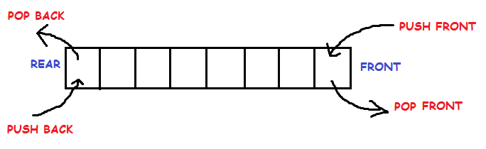
Implementation of Double ended Queue
Here we will implement a double ended queue using a circular array. It will have the following methods:
// Maximum size of array or Dequeue

#define SIZE 5

class Dequeue
{
    //front and rear to store the head and tail pointers
    int  *arr;
    int front, rear;

    public :

    Dequeue()
    {
    	//Create the array
        arr = new int[SIZE];

        //Initialize front and rear with -1
        front = -1;
        rear = -1;
    }

    // Operations on Deque
    void  push_front(int );
    void  push_back(int );
    void  pop_front();
    void  pop_back();
    int  get_front();
    int  get_back();
    bool  full();
    bool  empty();
};
Insert Elements at Front
First we check if the queue is full. If its not full we insert an element at front end by following the given conditions :
- If the queue is empty then intialize front and rear to 0. Both will point to the first element.
- Else we decrement front and insert the element. Since we are using circular array, we have to keep in mind that if front is equal to 0 then instead of decreasing it by 1 we make it equal to SIZE-1.
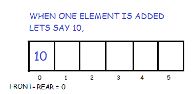
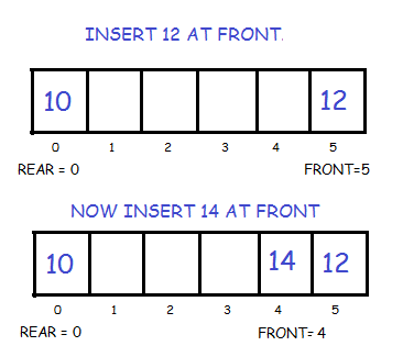
void Dequeue :: push_front(int key)
{
    if(full())
    {
        cout << "OVERFLOW\n";
    }
    else
    {
    	//If queue is empty
    	if(front == -1)
    		front = rear = 0;

    	//If front points to the first position element
        else if(front == 0)
            front = SIZE-1;

        else
        	--front;

        arr[front] = key;
    }
}
Insert Elements at back
Again we check if the queue is full. If its not full we insert an element at back by following the given conditions:
- If the queue is empty then intialize front and rear to 0. Both will point to the first element.
- Else we increment rear and insert the element. Since we are using circular array, we have to keep in mind that if rear is equal to SIZE-1 then instead of increasing it by 1 we make it equal to 0.
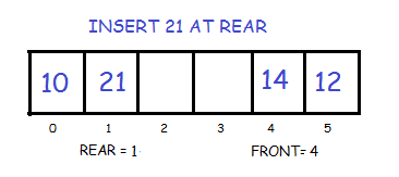
void Dequeue :: push_back(int key)
{
    if(full())
    {
        cout << "OVERFLOW\n";
    }
    else
    {
        //If queue is empty
    	   if(front == -1)
    		  front = rear = 0;

    	   //If rear points to the last element
        else if(rear == SIZE-1)
            rear = 0;

        else
        	++rear;

        arr[rear] = key;
    }
}
Delete First Element
In order to do this, we first check if the queue is empty. If its not then delete the front element by following the given conditions :
- If only one element is present we once again make front and rear equal to -1.
- Else we increment front. But we have to keep in mind that if front is equal to SIZE-1 then instead of increasing it by 1 we make it equal to 0.
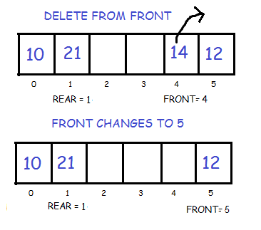
void Dequeue :: pop_front()
{
    if(empty())
    {
        cout << "UNDERFLOW\n";
    }
    else
    {
    	//If only one element is present
        if(front == rear)
        	front = rear = -1;

        //If front points to the last element
        else if(front == SIZE-1)
        	front = 0;

        else
        	++front;
    }
}
Delete Last Element
Inorder to do this, we again first check if the queue is empty. If its not then we delete the last element by following the given conditions :
- If only one element is present we make front and rear equal to -1.
- Else we decrement rear. But we have to keep in mind that if rear is equal to 0 then instead of decreasing it by 1 we make it equal to SIZE-1.
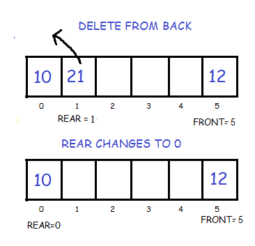
void Dequeue :: pop_back()
{
    if(empty())
    {
        cout << "UNDERFLOW\n";
    }
    else
    {
    	//If only one element is present
        if(front == rear)
        	front = rear = -1;

        //If rear points to the first position element
        else if(rear == 0)
        	rear = SIZE-1;

        else
        	--rear;
    }
}
Check if Queue is empty
It can be simply checked by looking where front points to. If front is still intialized with -1, the queue is empty.
bool Dequeue :: empty()
{
    if(front == -1)
    	return true;
    else
    	return false;
}
Check if Queue is full
Since we are using circular array, we check for following conditions as shown in code to check if queue is full.
bool Dequeue :: full()
{
    if((front == 0 && rear == SIZE-1)  ||
    	(front == rear + 1))
        return true;
    else
        return false;
}
Return First Element
If the queue is not empty then we simply return the value stored in the position which front points.
int Dequeue :: get_front()
{
    if(empty())
    {	cout << "f=" <<front << endl;
        cout << "UNDERFLOW\n";
        return -1;
    }
    else
    {
        return arr[front];
    }
}
Return Last Element
If the queue is not empty then we simply return the value stored in the position which rear points.
int Dequeue :: get_back()
{
    if(empty())
    {
        cout << "UNDERFLOW\n";
        return -1;
    }
    else
    {
        return arr[rear];
    }
}
Stack using Queue
A Stack is a Last In First Out(LIFO) structure, i.e, the element that is added last in the stack is taken out first. Our goal is to implement a Stack using Queue for which will be using two queues and design them in such a way that pop operation is same as dequeue but the push operation will be a little complex and more expensive too.
Implementation of Stack using Queue
Assuming we already have a class implemented for Queue, we first design the class for Stack. It will have the methods push() and pop() and two queues.
class Stack
{
	public:
	// two queue
	Queue Q1, Q2;
	// push method to add data element
	void push(int);
	// pop method to remove data element
	void pop();
};
Inserting Data in Stack
Since we are using Queue which is First In First Out(FIFO) structure , i.e, the element which is added first is taken out first, so we will implement the push operation in such a way that whenever there is a pop operation, the stack always pops out the last element added.
In order to do so, we will require two queues, Q1 and Q2. Whenever the push operation is invoked, we will enqueue(move in this case) all the elements of Q1 to Q2 and then enqueue the new element to Q1. After this we will enqueue(move in this case) all the elements from Q2 back to Q1.
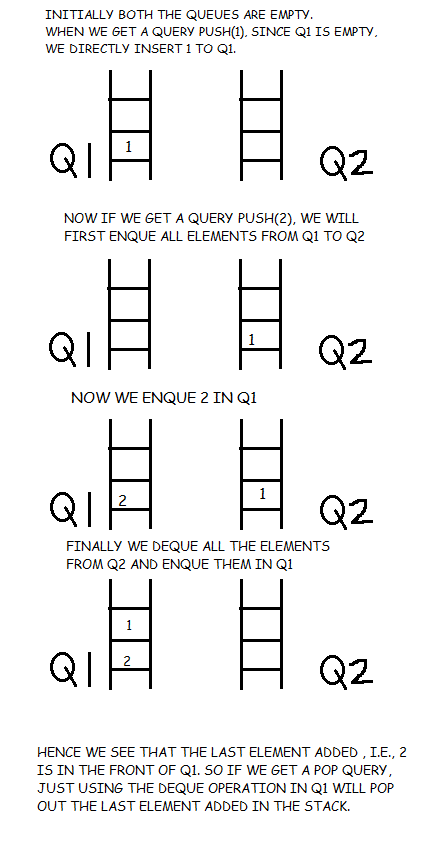
So let's implement this in our code,
void Stack :: push(int x)
{
	// move all elements in Q1 to Q2
	while(!Q1.isEmpty())
	{
		int temp = Q1.deque();
		Q2.enque(temp);
	}

	// add the element which is pushed into Stack
	Q1.enque(x);

	// move back all elements back to Q1 from Q2
	while(!Q2.isEmpty())
	{
		int temp = Q2.deque();
		Q1.enque(temp);
	}
}
It must be clear to you now, why we are using two queues. Actually the queue Q2 is just for the purpose of keeping the data temporarily while operations are executed.
In this way we can ensure that whenever the pop operation is invoked, the stack always pops out the last element added in Q1 queue.
Removing Data from Stack
Like we have discussed above, we just need to use the dequeue operation on our queue Q1. This will give us the last element added in Stack.
int Stack :: pop()
{
	return Q1.deque();
}
Time Complexity Analysis
When we implement Stack using a Queue the push operation becomes expensive.
- Push operation: O(n)
- Pop operation: O(1)
Conclusion
When we say "implementing Stack using Queue", we mean how we can make a Queue behave like a Stack, after all they are all logical entities. So for any data structure to act as a Stack, it should have push() method to add data on top and pop() method to remove data from top. Which is exactly what we did and hence accomplished to make a Queue(in this case two Queues) behave as a Stack.
Stack using Linked List
Stack as we know is a Last In First Out(LIFO) data structure. It has the following operations :
- push: push an element into the stack
- pop: remove the last element added
- top: returns the element at top of stack
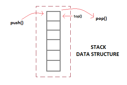
Implementation of Stack using Linked List
Stacks can be easily implemented using a linked list. Stack is a data structure to which a data can be added using the push() method and data can be removed from it using the pop() method. With Linked list, the push operation can be replaced by the addAtFront() method of linked list and pop operation can be replaced by a function which deletes the front node of the linked list.
In this way our Linked list will virtually become a Stack with push() and pop() methods.
First we create a class node. This is our Linked list node class which will have data in it and a node pointer to store the address of the next node element.
class node
{
	int data;
	node *next;
};
Then we define our stack class,
class Stack
{
	node *front;  // points to the head of list
	public:
	Stack()
	{
		front = NULL;
	}
	// push method to add data element
	void push(int);
	// pop method to remove data element
	void pop();
	// top method to return top data element
	int top();
};
Inserting Data in Stack (Linked List)
In order to insert an element into the stack, we will create a node and place it in front of the list.
void Stack :: push(int d)
{
	// creating a new node
	node *temp;
	temp = new node();
	// setting data to it
	temp->data = d;

	// add the node in front of list
	if(front == NULL)
	{
		temp->next = NULL;
	}
	else
	{
		temp->next = front;
	}
	front = temp;
}
Now whenever we will call the push() function a new node will get added to our list in the front, which is exactly how a stack behaves.
Removing Element from Stack (Linked List)
In order to do this, we will simply delete the first node, and make the second node, the head of the list.
void Stack :: pop()
{
	// if empty
	if(front == NULL)
		cout << "UNDERFLOW\n";

	// delete the first element
	else
	{
		node *temp = front;
		front = front->next;
		delete(temp);
	}
}
Return Top of Stack (Linked List)
In this, we simply return the data stored in the head of the list.
int Stack :: top()
{
	return front->data;
}
Conclusion
When we say "implementing Stack using Linked List", we mean how we can make a Linked List behave like a Stack, after all they are all logical entities. So for any data structure to act as a Stack, it should have push() method to add data on top and pop() method to remove data from top. Which is exactly what we did and hence accomplished to make a Linked List behave as a Stack.
Doubly Linked List
Doubly linked list is a type of linked list in which each node apart from storing its data has two links. The first link points to the previous node in the list and the second link points to the next node in the list. The first node of the list has its previous link pointing to NULL similarly the last node of the list has its next node pointing to NULL.
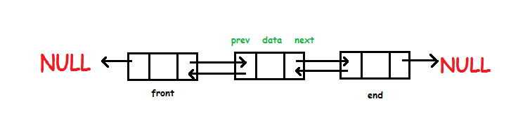
The two links help us to traverse the list in both backward and forward direction. But storing an extra link requires some extra space.
Implementation of Doubly Linked List
First we define the node.
struct node
{
	int data;     	// Data
	node *prev;  	// A reference to the previous node
	node *next; 	// A reference to the next node
};
Now we define our class Doubly Linked List. It has the following methods:
- add_front: Adds a new node in the beginning of list
- add_after: Adds a new node after another node
- add_before: Adds a new node before another node
- add_end: Adds a new node in the end of list
- delete: Removes the node
- forward_traverse: Traverse the list in forward direction
- backward_traverse: Traverse the list in backward direction
class Doubly_Linked_List
{
	node *front;  	// points to first node of list
	node *end;   	// points to first las of list
	public:
	Doubly_Linked_List()
	{
		front = NULL;
		end = NULL;
	}
	void add_front(int );
	void add_after(node* , int );
	void add_before(node* , int );
	void add_end(int );
	void delete_node(node*);
	void forward_traverse();
	void backward_traverse();
};
Insert Data in the beginning
- The prev pointer of first node will always be NULL and next will point to front.
- If the node is inserted is the first node of the list then we make front and end point to this node.
- Else we only make front point to this node.
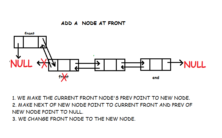
void Doubly_Linked_List :: add_front(int d)
{
	// Creating new node
	node *temp;
	temp = new node();
	temp->data = d;
	temp->prev = NULL;
	temp->next = front;

	// List is empty
	if(front == NULL)
		end = temp;

	else
		front->prev = temp;

	front = temp;
}
Insert Data before a Node
Let’s say we are inserting node X before Y. Then X’s next pointer will point to Y and X’s prev pointer will point the node Y’s prev pointer is pointing. And Y’s prev pointer will now point to X. We need to make sure that if Y is the first node of list then after adding X we make front point to X.
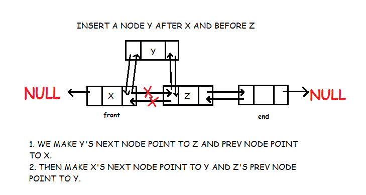
void Doubly_Linked_List :: add_before(node *n, int d)
{
	node *temp;
	temp = new node();
	temp->data = d;
	temp->next = n;
	temp->prev = n->prev;
	n->prev = temp;

	//if node is to be inserted before first node
	if(n->prev == NULL)
		front = temp;
}
Insert Data after a Node
Let’s say we are inserting node Y after X. Then Y’s prev pointer will point to X and Y’s next pointer will point the node X’s next pointer is pointing. And X’s next pointer will now point to Y. We need to make sure that if X is the last node of list then after adding Y we make end point to Y.
void Doubly_Linked_List :: add_after(node *n, int d)
{
	node *temp;
	temp = new node();
	temp->data = d;
	temp->prev = n;
	temp->next = n->next;
	n->next = temp;

	//if node is to be inserted after last node
	if(n->next == NULL)
		end = temp;
}
Insert Data in the end
- The next pointer of last node will always be NULL and prev will point to end.
- If the node is inserted is the first node of the list then we make front and end point to this node.
- Else we only make end point to this node.
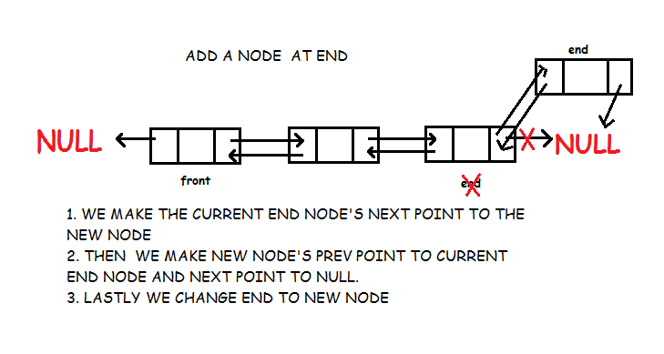
void Doubly_Linked_List :: add_end(int d)
{
	// create new node
	node *temp;
	temp = new node();
	temp->data = d;
	temp->prev = end;
	temp->next = NULL;

	// if list is empty
	if(end == NULL)
		front = temp;
	else
		end->next = temp;
	end = temp;
}
Remove a Node
Removal of a node is quite easy in Doubly linked list but requires special handling if the node to be deleted is first or last element of the list. Unlike singly linked list where we require the previous node, here only the node to be deleted is needed. We simply make the next of the previous node point to next of current node (node to be deleted) and prev of next node point to prev of current node. Look code for more details.
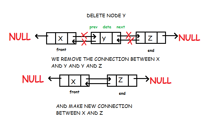
void Doubly_Linked_List :: delete_node(node *n)
{
	// if node to be deleted is first node of list
	if(n->prev == NULL)
	{
		front = n->next; //the next node will be front of list
		front->prev = NULL;
	}
	// if node to be deleted is last node of list
	else if(n->next == NULL)
	{
		end = n->prev;   // the previous node will be last of list
		end->next = NULL;
	}
	else
	{
		//previous node's next will point to current node's next
		n->prev->next = n->next;
		//next node's prev will point to current node's prev
		n->next->prev = n->prev;
	}
	//delete node
	delete(n);
}
Forward Traversal
Start with the front node and visit all the nodes untill the node becomes NULL.
void Doubly_Linked_List :: forward_traverse()
{
	node *trav;
	trav = front;
	while(trav != NULL)
	{
		cout<<trav->data<<endl;
		trav = trav->next;
	}
}
Backward Traversal
Start with the end node and visit all the nodes until the node becomes NULL.
void Doubly_Linked_List :: backward_traverse()
{
	node *trav;
	trav = end;
	while(trav != NULL)
	{
		cout<<trav->data<<endl;
		trav = trav->prev;
	}
}- Pointer to left subtree
- Pointer to right subtree
- Data element
- Root: Topmost node in a tree.
- Parent: Every node (excluding a root) in a tree is connected by a directed edge from exactly one other node. This node is called a parent.
- Child: A node directly connected to another node when moving away from the root.
- Leaf/External node: Node with no children.
- Internal node: Node with atleast one children.
- Depth of a node: Number of edges from root to the node.
- Height of a node: Number of edges from the node to the deepest leaf. Height of the tree is the height of the root.
- Trees reflect structural relationships in the data.
- Trees are used to represent hierarchies.
- Trees provide an efficient insertion and searching.
- Trees are very flexible data, allowing to move subtrees around with minumum effort.
- Rooted binary tree: It has a root node and every node has atmost two children.
- Full binary tree: It is a tree in which every node in the tree has either 0 or 2 children.
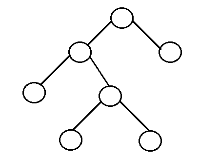
- The number of nodes, n, in a full binary tree is atleast n = 2h – 1, and atmost n = 2h+1 – 1, where h is the height of the tree.
- The number of leaf nodes l, in a full binary tree is number, L of internal nodes + 1, i.e, l = L+1.
- Perfect binary tree: It is a binary tree in which all interior nodes have two children and all leaves have the same depth or same level.
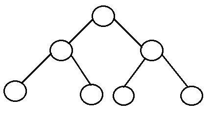
- A perfect binary tree with l leaves has n = 2l-1 nodes.
- In perfect full binary tree, l = 2h and n = 2h+1 - 1 where, n is number of nodes, h is height of tree and l is number of leaf nodes
- Complete binary tree: It is a binary tree in which every level, except possibly the last, is completely filled, and all nodes are as far left as possible.
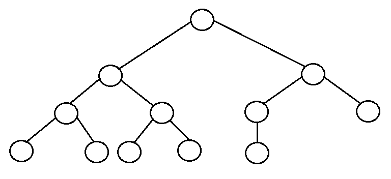
- The number of internal nodes in a complete binary tree of n nodes is floor(n/2).
- Balanced binary tree: A binary tree is height balanced if it satisfies the following constraints:
- The left and right subtrees' heights differ by at most one, AND
- The left subtree is balanced, AND
- The right subtree is balanced
An empty tree is height balanced.
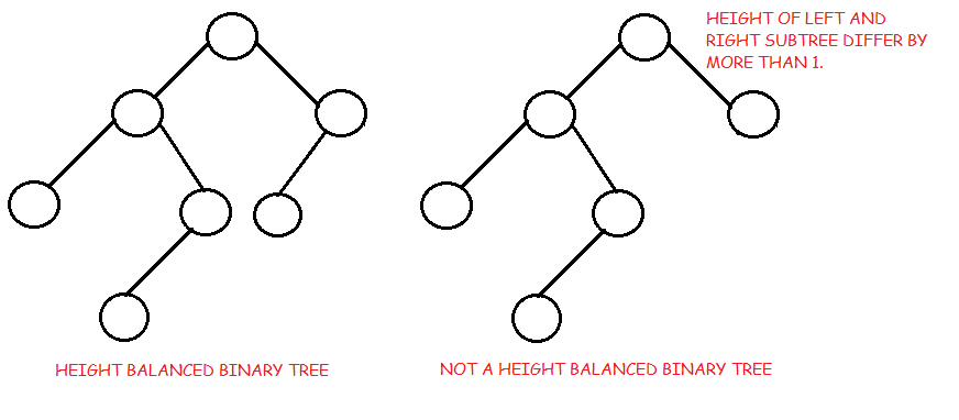
- The height of a balanced binary tree is O(Log n) where n is number of nodes.
- Degenarate tree: It is a tree is where each parent node has only one child node. It behaves like a linked list.
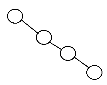
Introduction To Binary Trees
A binary tree is a hierarchical data structure in which each node has at most two children generally referred as left child and right child.
Each node contains three components:
The topmost node in the tree is called the root. An empty tree is represented by NULL pointer.
A representation of binary tree is shown:
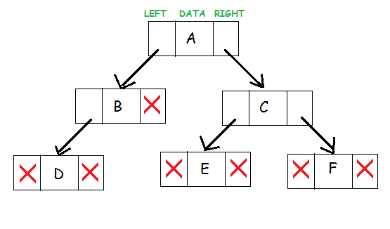
Binary Tree: Common Terminologies
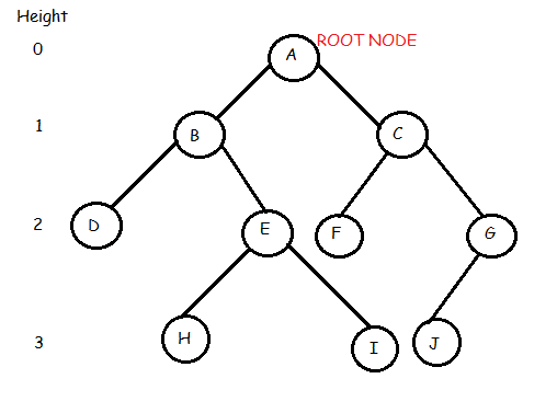
In the above binary tree we see that root node is A. The tree has 10 nodes with 5 internal nodes, i.e, A,B,C,E,G and 5 external nodes, i.e, D,F,H,I,J. The height of the tree is 3. B is the parent of D and E while D and E are children of B.
Advantages of Trees
Trees are so useful and frequently used, because they have some very serious advantages:
Types of Binary Trees (Based on Structure)
Binary Search Tree
A binary search tree is a useful data structure for fast addition and removal of data.
It is composed of nodes, which stores data and also links to upto two other child nodes. It is the relationship between the leaves linked to and the linking leaf, also known as the parent node, which makes the binary tree such an efficient data structure.
For a binary tree to be a binary search tree, the data of all the nodes in the left sub-tree of the root node should be less than the data of the root. The data of all the nodes in the right subtree of the root node should be greater than equal to the data of the root. As a result, the leaves on the farthest left of the tree have the lowest values, whereas the leaves on the right of the tree have the greatest values.
A representation of binary search tree looks like the following:
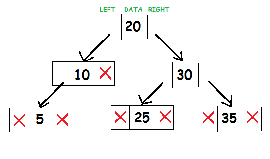
Consider the root node 20. All elements to the left of subtree(10, 5) are less than 20 and all elements to the right of subtree(25, 30, 35) are greater than 20.
Implementation of BST
First, define a struct as tree_node. It will store the data and pointers to left and right subtree.
struct tree_node
{
	int data;
	tree_node *left, *right;
};
The node itself is very similar to the node in a linked list. A basic knowledge of the code for a linked list will be very helpful in understanding the techniques of binary trees.
It is most logical to create a binary search tree class to encapsulate the workings of the tree into a single area, and also making it reusable. The class will contain functions to insert data into the tree, search if the data is present and methods for traversing the tree.
class BST
{
	tree_node *root;
	void insert(tree_node* , int );
	bool search(int , tree_node* );
	void inorder(tree_node* );
	void preorder(tree_node* );
	void postorder(tree_node* );

	public:
	BST()
	{
		root = NULL;
	}
	void insert(int );
	bool search(int key);
    void inorder();
    void preorder();
    void postorder();
};
It is necessary to initialize root to NULL for the later functions to be able to recognize that it does not exist.
All the public members of the class are designed to allow the user of the class to use the class without dealing with the underlying design. The functions which will be called recursively are the ones which are private, allowing them to travel down the tree.
Insertion in a BST
To insert data into a binary tree involves a function searching for an unused node in the proper position in the tree in which to insert the key value. The insert function is generally a recursive function that continues moving down the levels of a binary tree until there is an unused leaf in a position which follows the following rules of placing nodes.
- Compare data of the root node and element to be inserted.
- If the data of the root node is greater, and if a left subtree exists, then repeat step 1 with root = root of left subtree. Else,
- Insert element as left child of current root.
- If the data of the root node is greater, and if a right subtree exists, then repeat step 1 with root = root of right subtree.
- Else, insert element as right child of current root.
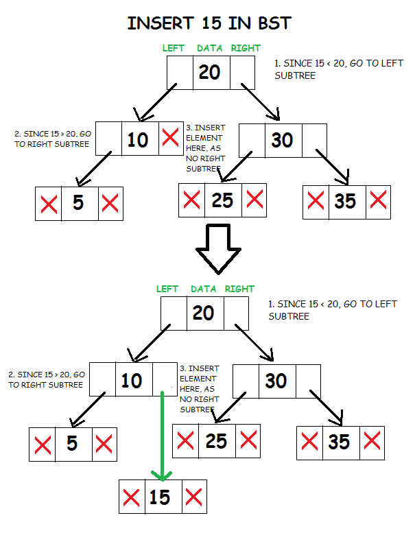
void BST :: insert(tree_node *node, int d)
{
	// element to be inserted is lesser than node’s data
	if(d < node->data)
	{
		// if left subtree is present
		if(node->left != NULL)
			insert(node->left, d);

		// create new node
		else
		{
			node->left = new tree_node;
			node->left->data = d;
			node->left->left = NULL;
			node->left->right = NULL;
		}
	}

	// element to be inserted is greater than node’s data
	else if(d >= node->data)
	{
		// if left subtree is present
		if(node->right != NULL)
			insert(node->right, d);

		// create new node
		else
		{
			node->right = new tree_node;
			node->right->data = d;
			node->right->left = NULL;
			node->right->right = NULL;
		}
	}

}
Since the root node is a private member, we also write a public member function which is available to non-members of the class. It calls the private recursive function to insert an element and also takes care of the case when root node is NULL.
void BST::insert(int d)
{
	if(root!=NULL)
                insert(root, d);
	else
    {
        root = new tree_node;
        root->data = d;
        root->left = NULL;
        root->right = NULL;
    }
}
Searching in a BST
The search function works in a similar fashion as insert. It will check if the key value of the current node is the value to be searched. If not, it should check to see if the value to be searched for is less than the value of the node, in which case it should be recursively called on the left child node, or if it is greater than the value of the node, it should be recursively called on the right child node.
- Compare data of the root node and the value to be searched.
- If the data of the root node is greater, and if a left subtree exists, then repeat step 1 with root = root of left subtree. Else,
- If the data of the root node is greater, and if a right subtree exists, then repeat step 1 with root = root of right subtree. Else,
- If the value to be searched is equal to the data of root node, return true.
- Else, return false.
bool BST::search(int d, tree_node *node)
{
	bool ans = false;

	// node is not present
  	if(node == NULL)
 		return false;

	// Node’s data is equal to value searched
    if(d == node->data)
      	return true;

	// Node’s data is greater than value searched
    else if(d < node->data)
       	ans = search(d, node->left);

	// Node’s data is lesser than value searched
    else
       	ans = search(d, node->right);

    return ans;
}
Since the root node is a private member, we also write a public member function which is available to non-members of the class. It calls the private recursive function to search an element and also takes care of the case when root node is NULL.
bool BST::search(int d)
{
	if(root ==  NULL)
		return false;
	else
		return  search(d, root);
}
Traversing in a BST
There are mainly three types of tree traversals:
1. Pre-order Traversal:
In this technique, we do the following :
- Process data of root node.
- First, traverse left subtree completely.
- Then, traverse right subtree.
void BST :: preorder(tree_node *node)
{
	if(node !=  NULL)
    {
		cout<<node->data<<endl;
       	preorder(node->left);
       	preorder(node->right);
    }
}
2. Post-order Traversal
In this traversal technique we do the following:
- First traverse left subtree completely.
- Then, traverse right subtree completely.
- Then, process data of node.
void BST :: postorder(tree_node *node)
{
	if(node !=  NULL)
   	{
        postorder(node->left);
        postorder(node->right);
	    cout<<node->data<<endl;
   	}
}
3. In-order Traversal
In in-order traversal, we do the following:
- First process left subtree.
- Then, process current root node.
- Then, process right subtree.
void BST :: inorder(tree_node *node)
{
	if(node !=  NULL)
   	{
        inorder(node->left);
	    cout<<node->data<<endl;
        inorder(node->right);
   	}
}
The in-order traversal of a binary search tree gives a sorted ordering of the data elements that are present in the binary search tree. This is an important property of a binary search tree.
Since the root node is a private member, we also write public member functions which is available to non-members of the class. It calls the private recursive function to traverse the tree and also takes care of the case when root node is NULL.
void BST :: preorder()
{
	if(root ==  NULL)
		cout<<"TREE IS  EMPTY\n";
	else
       	preorder(root);
}

void BST :: postorder()
{
	if(root ==  NULL)
		cout<<"TREE IS  EMPTY\n";
	else
	    postorder(root);
}

void BST :: inorder()
{
	if(root == NULL)
		cout<<"TREE IS EMPTY\n";
	else
		inorder(root);
}
Complexity Analysis
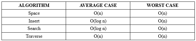
The time complexity of search and insert rely on the height of the tree. On average, binary search trees with n nodes have O(log n) height. However in the worst case the tree can have a height of O(n) when the unbalanced tree resembles a linked list. For example in this case :
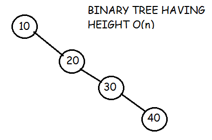
Traversal requires O(n) time, since every node must be visited.
Greedy Approach or Technique
As the name implies, this is a simple approach which tries to find the best solution at every step. Thus, it aims to find the local optimal solution at every step so as to find the global optimal solution for the entire problem.
Consider that there is an objective function that has to be optimized (maximized/ minimized). This approach makes greedy choices at each step and makes sure that the objective function is optimized.
The greedy algorithm has only one chance to compute the optimal solution and thus, cannot go back and look at other alternate solutions. However, in many problems, this strategy fails to produce a global optimal solution. Let's consider the following binary tree to understand how a basic greedy algorithm works:
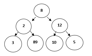
For the above problem the objective function is:
To find the path with largest sum.
Since we need to maximize the objective function, Greedy approach can be used. Following steps are followed to find the solution:
Step 1: Initialize sum = 0
Step 2: Select the root node, so its value will be added to sum, sum = 0+8 = 8
Step 3: The algorithm compares nodes at next level, selects the largest node which is 12, making the sum = 20.
Step 4: The algorithm compares nodes at the next level, selects the largest node which is 10, making the sum = 30.
Thus, using the greedy algorithm, we get 8-12-10 as the path. But this is not the optimal solution, since the path 8-2-89 has the largest sum ie 99.
This happens because the algorithm makes decision based on the information available at each step without considering the overall problem.
When to use Greedy Algorithms?
For a problem with the following properties, we can use the greedy technique:
Greedy Choice Property: This states that a globally optimal solution can be obtained by locally optimal choices.
Optimal Sub-Problem: This property states that an optimal solution to a problem, contains within it, optimal solution to the sub-problems. Thus, a globally optimal solution can be constructed from locally optimal sub-solutions.
Generally, optimization problem, or the problem where we have to find maximum or minimum of something or we have to find some optimal solution, greedy technique is used.
An optimization problem has two types of solutions:
Feasible Solution: This can be referred as approximate solution (subset of solution) satisfying the objective function and it may or may not build up to the optimal solution.
Optimal Solution: This can be defined as a feasible solution that either maximizes or minimizes the objective function.
Key Terminologies used in Greedy Algorithms
Objective Function: This can be defined as the function that needs to be either maximized or minimized.
Candidate Set: The global optimal solution is created from this set.
Selection Function: Determines the best candidate and includes it in the solution set.
Feasibility Function: Determines whether a candidate is feasible and can contribute to the solution.
Standard Greedy Algorithm
This algorithm proceeds step-by-step, considering one input, say x, at each step.
- If
xgives a local optimal solution (xis feasible), then it is included in the partial solution set, else it is discarded. - The algorithm then goes to the next step and never considers
xagain. - This continues until the input set is finished or the optimal solution is found.
The above algorithm can be translated into the following pseudocode:
Algorithm Greedy(a, n)   // n defines the input set
{
    solution= NULL;		// initialize solution set
	for i=1 to n do
	{
		x = Select(a);	// Selection Function
		if Feasible(solution, x) then 	// Feasibility solution
			solution = Union (solution, x);   // Include x in the solution set
	}
	return solution;
}
Advantages of Greedy Approach/Technique
- This technique is easy to formulate and implement.
- It works efficiently in many scenarios.
- This approach minimizes the time required for generating the solution.
Now, let's see a few disadvantages too,
Disadvantages of Greedy Approach/Technique
- This approach does not guarantee a global optimal solution since it never looks back at the choices made for finding the local optimal solution.
Although we have already covered that which type of problem in general can be solved using greedy approach, here are a few popular problems which use greedy technique:
- Knapsack Problem
- Activity Selection Problem
- Dijkstra’s Problem
- Prim’s Algorithmfor finding Minimum Spanning Tree
- Kruskal’s Algorithmfor finding Minimum Spanning Tree
- Huffman Coding
- Travelling Salesman Problem
Conclusion
Greedy Technique is best suited for applications where:
- Solution is required in real-time.
- Approximate solution is sufficient.
- It might not be possible to complete all the activities, since their timings can collapse.
- Two activities, say i and j, are said to be non-conflicting if
si >= fjorsj >= fiwheresiandsjdenote the starting time of activities i and j respectively, andfiandfjrefer to the finishing time of the activities i and j respectively. - Greedy approach can be used to find the solution since we want to maximize the count of activities that can be executed. This approach will greedily choose an activity with earliest finish time at every step, thus yielding an optimal solution.
act[]array containing all the activities.s[]array containing the starting time of all the activities.f[]array containing the finishing time of all the activities.sol[]array refering to the solution set containing the maximum number of non-conflicting activities.- Select activity a3. Since the start time of a3 is greater than the finish time of a2 (i.e.
s(a3) > f(a2)), we add a3 to the solution set. Thus sol = {a2, a3}. - Select a4. Since
s(a4) < f(a3), it is not added to the solution set. - Select a5. Since
s(a5) > f(a3), a5 gets added to solution set. Thus sol = {a2, a3, a5} - Select a1. Since
s(a1) < f(a5), a1 is not added to the solution set. - Select a6. a6 is added to the solution set since
s(a6) > f(a5). Thus sol = {a2, a3, a5, a6}.
Activity Selection Problem
The Activity Selection Problem is an optimization problem which deals with the selection of non-conflicting activities that needs to be executed by a single person or machine in a given time frame.
Each activity is marked by a start and finish time. Greedy technique is used for finding the solution since this is an optimization problem.
What is Activity Selection Problem?
Let's consider that you have n activities with their start and finish times, the objective is to find solution set having maximum number of non-conflicting activities that can be executed in a single time frame, assuming that only one person or machine is available for execution.
Some points to note here:
Input Data for the Algorithm:
Ouput Data from the Algorithm:
Steps for Activity Selection Problem
Following are the steps we will be following to solve the activity selection problem,
Step 1: Sort the given activities in ascending order according to their finishing time.
Step 2: Select the first activity from sorted array act[] and add it to sol[] array.
Step 3: Repeat steps 4 and 5 for the remaining activities in act[].
Step 4: If the start time of the currently selected activity is greater than or equal to the finish time of previously selected activity, then add it to the sol[] array.
Step 5: Select the next activity in act[] array.
Step 6: Print the sol[] array.
Activity Selection Problem Example
Let's try to trace the steps of above algorithm using an example:
In the table below, we have 6 activities with corresponding start and end time, the objective is to compute an execution schedule having maximum number of non-conflicting activities:
| Start Time (s) | Finish Time (f) | Activity Name |
| 5 | 9 | a1 |
| 1 | 2 | a2 |
| 3 | 4 | a3 |
| 0 | 6 | a4 |
| 5 | 7 | a5 |
| 8 | 9 | a6 |
A possible solution would be:
Step 1: Sort the given activities in ascending order according to their finishing time.
The table after we have sorted it:
| Start Time (s) | Finish Time (f) | Activity Name |
| 1 | 2 | a2 |
| 3 | 4 | a3 |
| 0 | 6 | a4 |
| 5 | 7 | a5 |
| 5 | 9 | a1 |
| 8 | 9 | a6 |
Step 2: Select the first activity from sorted array act[] and add it to the sol[] array, thus sol = {a2}.
Step 3: Repeat the steps 4 and 5 for the remaining activities in act[].
Step 4: If the start time of the currently selected activity is greater than or equal to the finish time of the previously selected activity, then add it to sol[].
Step 5: Select the next activity in act[]
For the data given in the above table,
Step 6: At last, print the array sol[]
Hence, the execution schedule of maximum number of non-conflicting activities will be:
(1,2) (3,4) (5,7) (8,9)
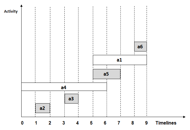
In the above diagram, the selected activities have been highlighted in grey.
Implementation of Activity Selection Problem Algorithm
Now that we have an overall understanding of the activity selection problem as we have already discussed the algorithm and its working details with the help of an example, following is the C++ implementation for the same.
Note: The algorithm can be easily written in any programming language.
#include <bits/stdc++.h>

using namespace std;
#define N 6		// defines the number of activities

// Structure represents an activity having start time and finish time.
struct Activity
{
    int start, finish;
};

// This function is used for sorting activities according to finish time
bool Sort_activity(Activity s1, Activity s2)
{
    return (s1.finish< s2.finish);
}

/* 	Prints maximum number of activities that can
	be done by a single person or single machine at a time.
*/
void print_Max_Activities(Activity arr[], int n)
{
    // Sort activities according to finish time
	sort(arr, arr+n, Sort_activity);

	cout<< "Following activities are selected \n";

    // Select the first activity
    int i = 0;
	cout<< "(" <<arr[i].start<< ", " <<arr[i].finish << ")\n";

    // Consider the remaining activities from 1 to n-1
    for (int j = 1; j < n; j++)
    {
    	// Select this activity if it has start time greater than or equal
    	// to the finish time of previously selected activity
      	if (arr[j].start>= arr[i].finish)
      	{
			cout<< "(" <<arr[j].start<< ", "<<arr[j].finish << ") \n";
			i = j;
      	}
    }
}

// Driver program
int main()
{
    Activity arr[N];
	for(int i=0; i<=N-1; i++)
	{
		cout<<"Enter the start and end time of "<<i+1<<" activity \n";
		cin>>arr[i].start>>arr[i].finish;
    }

	print_Max_Activities(arr, N);
    return 0;
}
The program is executed using same inputs as that of the example explained above. This will help in verifying the resultant solution set with actual output.
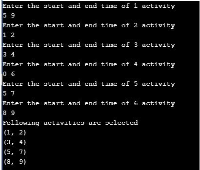
Time Complexity Analysis
Following are the scenarios for computing the time complexity of Activity Selection Algorithm:
- Case 1: When a given set of activities are already sorted according to their finishing time, then there is no sorting mechanism involved, in such a case the complexity of the algorithm will be
O(n) - Case 2: When a given set of activities is unsorted, then we will have to use the
sort()method defined in bits/stdc++ header file for sorting the activities list. The time complexity of this method will beO(nlogn), which also defines complexity of the algorithm.
Real-life Applications of Activity Selection Problem
Following are some of the real-life applications of this problem:
- Scheduling multiple competing events in a room, such that each event has its own start and end time.
- Scheduling manufacturing of multiple products on the same machine, such that each product has its own production timelines.
- Activity Selection is one of the most well-known generic problems used in Operations Research for dealing with real-life business problems
Prim's Minimum Spanning Tree
In this tutorial we will cover another algorithm which uses greedy approach/technique for finding the solution.
Let's start with a real-life scenario to understant the premise of this algorithm:
- A telecommunications organization, has offices spanned across multiple locations around the globe.
 Figure 1
 - It has to use leased phone lines for connecting all these offices with each other.
- The cost(in units) of connecting each pair of offices is different and is shown as follows:
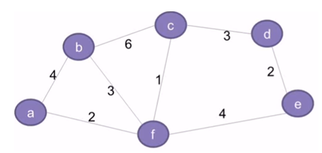 Figure 2
 - The organization, thus, wants to use minimum cost for connecting all its offices. This requires that all the offices should be connected using minimum number of leased lines so as to reduce the effective cost.
- The solution to this problem can be implemented by using the concept of Minimum Spanning Tree, which is discussed in the subsequent section.
- This tutorial also details the concepts related to Prim's Algorithm which is used for finding the minimum spanning tree for a given graph.
What is a Spanning Tree?
The network shown in the second figure basically represents a graph G = (V, E) with a set of vertices V = {a, b, c, d, e, f} and a set of edges E = { (a,b), (b,c), (c,d), (d,e), (e,f), (f,a), (b,f), (c,f) }. The graph is:
- Connected (there exists a path between every pair of vertices)
- Undirected (the edges do no have any directions associated with them such that (a,b) and (b,a) are equivalent)
- Weighted (each edge has a weight or cost assigned to it)
A spanning tree G' = (V, E') for the given graph G will include:
- All the vertices (V) of G
- All the vertices should be connected by minimum number of edges (E') such that
E' ⊂ E - G' can have maximum
n-1edges, wherenis equal to the total number of edges in G - G' should not have any cycles. This is one of the basic differences between a tree and graph that a graph can have cycles, but a tree cannot. Thus, a tree is also defined as an acyclic graph.
Following is an example of a spanning tree for the above graph. Please note that only the highlighted edges are included in the spanning tree,
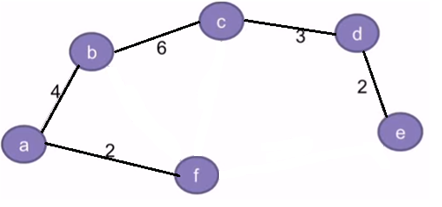 Figure 3
Also, there can be multiple spanning trees possible for any given graph. For eg: In addition to the spanning tree in the above diagram, the graph can also have another spanning tree as shown below:
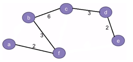 Figure 4
By convention, the total number of spanning trees for a given graph can be defined as:
nCm = n!/(m!*(n-m)!), where,
nis equal to the total number of edges in the given graphmis equal to the total number of edges in the spanning tree such thatm <= (n-1).
Hence, the total number of spanning trees(S) for the given graph(second diagram from top) can be computed as follows:
- n = 8, for the given graph in Fig. 2
- m = 5, since its corresponding spanning tree can have only 5 edges. Adding a 6th edge can result in the formation of cycles which is not allowed.
- So, S = nCm = 8C5 = 8!/ (5! * 3!) = 56, which means that 56 different variations of spannig trees can be created for the given graph.
What is a Minimum Spanning Tree?
The cost of a spanning tree is the total of the weights of all the edges in the tree. For example, the cost of spanning tree in Fig. 3 is (2+4+6+3+2) = 17 units, whereas in Fig. 4 it is (2+3+6+3+2) = 16 units.
Since we can have multiple spanning trees for a graph, each having its own cost value, the objective is to find the spanning tree with minimum cost. This is called a Minimum Spanning Tree(MST).
Note: There can be multiple minimum spanning trees for a graph, if any two edges in the graph have the same weight. However, if each edge has a distinct weight, then there will be only one minimum spanning tree for any given graph.
Problem Statement for Minimum Spanning Tree
Given a weighted, undirected and connected graph G, the objective is to find the minimum spanning tree G' for G.
Apart from the Prim's Algorithm for minimum spanning tree, we also have Kruskal's Algorithm for finding minimum spanning tree.
However, this tutorial will only discuss the fundamentals of Prim's Algorithm.
Since this algorithm aims to find the spanning tree with minimum cost, it uses greedy approach for finding the solution.
As part of finding the or creating the minimum spanning tree fram a given graph we will be following these steps:
- Initially, the tree is empty.
- The tree starts building from a random source vertex.
- A new vertex gets added to the tree at every step.
- This continues till all the vertices of graph are added to the tree.
Input Data will be:
A Cost Adjacency Matrix for out graph G, say cost
Output will be:
A Spanning tree with minimum total cost
Algorithm for Prim's Minimum Spanning Tree
Below we have the complete logic, stepwise, which is followed in prim's algorithm:
Step 1: Keep a track of all the vertices that have been visited and added to the spanning tree.
Step 2: Initially the spanning tree is empty.
Step 3: Choose a random vertex, and add it to the spanning tree. This becomes the root node.
Step 4: Add a new vertex, say x, such that
- x is not in the already built spanning tree.
- x is connected to the built spanning tree using minimum weight edge. (Thus, x can be adjacent to any of the nodes that have already been added in the spanning tree).
- Adding x to the spanning tree should not form cycles.
Step 5: Repeat the Step 4, till all the vertices of the graph are added to the spanning tree.
Step 6: Print the total cost of the spanning tree.
Example for Prim's Minimum Spanning Tree Algorithm
Let's try to trace the above algorithm for finding the Minimum Spanning Tree for the graph in Fig. 2:
Step A:
- Define
key[]array for storing the key value(or cost) of every vertex. Initialize this to∞(infinity) for all the vertices - Define another array
booleanvisited[]for keeping a track of all the vertices that have been added to the spanning tree. Initially this will be 0 for all the vertices, since the spanning tree is empty. - Define an array
parent[]for keeping track of the parent vertex. Initialize this to -1 for all the vertices. - Initialize minimum cost, minCost = 0
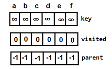 Figure 5: Initial arrays when tree is empty
Step B:
Choose any random vertex, say f and set key[f]=0.
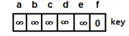 Figure 6: Setting key value of root node
Since its key value is minimum and it is not visited, add f to the spanning tree.
 Figure 7: Root Node
Also, update the following:
minCost = 0 + key[f] = 0- This is how the
visited[]array will look like: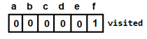 Figure 8: visited array after adding the root node
 - Key values for all the adjacent vertices of f will look like this(key value is nothing but the cost or the weight of the edge, for (f,d) it is still infinity because they are not directly connected):
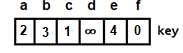 Figure 9: key array after adding the root node
Note: There will be no change in the parent[] because f is the root node.
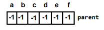 Figure 10: parent array after adding the root node
Step C:
The arrays key[] and visited[] will be searched for finding the next vertex.
- f has the minimum key value but will not be considered since it is already added (
visited[f]==1) - Next vertex having the minimum key value is c. Since
visited[c]==0, it will be added to the spanning tree.
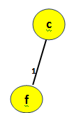 Figure 11: Adding vertex c
Again, update the following:
minCost = 0 + key[c] = 0 + 1 = 1- This is how the
visited[]array will look like: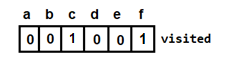 Figure 12: visited array after adding vertex c
 - And, the
parent[]array (f becomes the parent of c):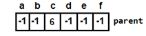 Figure 13: parent array after adding the root node
 - For every adjacent vertex of c, say v, values in
key[v]will be updated using the formula:key[v] = min(key[v], cost[c][v])Thus the
key[]array will become: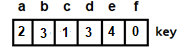 Figure 14: key array after adding the root node
Step D:
Repeat the Step C for the remaining vertices.
- Next vertex to be selected is a. And minimum cost will become
minCost=1+2=3 Figure 15: Adding vertex a
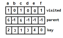 Figure 16: Updated arrays after adding vertex a
 - Next, either b or d can be selected. Let's consider b. Then the minimum cost will become
minCost=3+3=6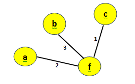 Figure 17: Adding vertex b to minimum spanning tree
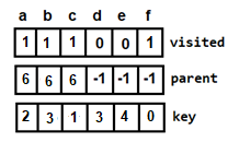 Figure 18: Updated arrays after adding vertex b
 - Next vertex to be selected is d, making the minimum cost
minCost=6+3=9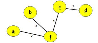 Figure 19: Adding vertex d
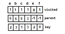 Figure 20: Updated arrays after adding vertex d
 - Then, e is selected and the minimum cost will become,
minCost=9+2=11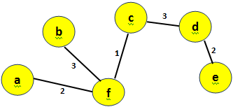 Figure 21: Adding vertex e. This is the final minimum spanning tree
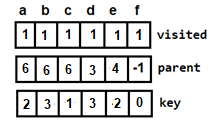 Figure 22: Updated arrays after adding vertex e (final arrays)
 - Since all the vertices have been visited now, the algorithm terminates.
- Thus, Fig. 21 represents the Minimum Spanning Tree with total cost=11.
Implementation of Prim's Minimum Spanning Tree Algorithm
Now it's time to write a program in C++ for the finding out minimum spanning tree using prim's algorithm.
#include<iostream>

using namespace std;

// Number of vertices in the graph
const int V=6;

// Function to find the vertex with minimum key value
int min_Key(int key[], bool visited[])
{
    int min = 999, min_index;  // 999 represents an Infinite value

    for (int v = 0; v < V; v++) {
        if (visited[v] == false && key[v] < min) {
        	// vertex should not be visited
            min = key[v];
			min_index = v;
        }
    }
    return min_index;
}

// Function to print the final MST stored in parent[]
int print_MST(int parent[], int cost[V][V])
{
    int minCost=0;
	cout<<"Edge \tWeight\n";
    for (int i = 1; i< V; i++) {
		cout<<parent[i]<<" - "<<i<<" \t"<<cost[i][parent[i]]<<" \n";
		minCost+=cost[i][parent[i]];
    }
	cout<<"Total cost is"<<minCost;
}

// Function to find the MST using adjacency cost matrix representation
void find_MST(int cost[V][V])
{
    int parent[V], key[V];
    bool visited[V];

    // Initialize all the arrays
    for (int i = 0; i< V; i++) {
        key[i] = 999;    // 99 represents an Infinite value
        visited[i] = false;
        parent[i]=-1;
    }

    key[0] = 0;  // Include first vertex in MST by setting its key vaue to 0.
    parent[0] = -1; // First node is always root of MST

    // The MST will have maximum V-1 vertices
    for (int x = 0; x < V - 1; x++)
    {
        // Finding the minimum key vertex from the
        //set of vertices not yet included in MST
        int u = min_Key(key, visited);

        visited[u] = true;  // Add the minimum key vertex to the MST

        // Update key and parent arrays
        for (int v = 0; v < V; v++)
        {
            // cost[u][v] is non zero only for adjacent vertices of u
            // visited[v] is false for vertices not yet included in MST
            // key[] gets updated only if cost[u][v] is smaller than key[v]
            if (cost[u][v]!=0 && visited[v] == false && cost[u][v] < key[v])
            {
                parent[v] = u;
                key[v] = cost[u][v];
            }
        }
    }

    // print the final MST
	print_MST(parent, cost);
}

// main function
int main()
{
    int cost[V][V];
	cout<<"Enter the vertices for a graph with 6 vetices";
    for (int i=0;i<V;i++)
    {
        for(int j=0;j<V;j++)
        {
			cin>>cost[i][j];
        }
    }
	find_MST(cost);

    return 0;
}
The input graph is the same as the graph in Fig 2.
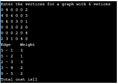 Figure 23: Output of the program
Time Complexity Analysis for Prim's MST
Time complexity of the above C++ program is O(V2) since it uses adjacency matrix representation for the input graph. However, using an adjacency list representation, with the help of binary heap, can reduce the complexity of Prim's algorithm to O(ElogV).
Real-world Applications of a Minimum Spanning Tree
Finding an MST is a fundamental problem and has the following real-life applications:
- Designing the networks including computer networks, telecommunication networks, transportation networks, electricity grid and water supply networks.
- Used in algorithms for approximately finding solutions to problems like Travelling Salesman problem, minimum cut problem, etc.
- The objective of a Travelling Salesman problem is to find the shortest route in a graph that visits each vertex only once and returns back to the source vertex.
- A minimum cut problem is used to find the minimum number of cuts between all the pairs of vertices in a planar graph. A graph can be classified as planar if it can be drawn in a plane with no edges crossing each other. For example,
 Figure 24: Planar Graph
- Also, a cut is a subset of edges which, if removed from a planar graph, increases the number of components in the graphFigure 25: Cut-Set in a Planar Graph
- Analysis of clusters.
- Handwriting recognition of mathematical expressions.
- Image registration and segmentation
Huffman Coding Algorithm
Every information in computer science is encoded as strings of 1s and 0s. The objective of information theory is to usually transmit information using fewest number of bits in such a way that every encoding is unambiguous. This tutorial discusses about fixed-length and variable-length encoding along with Huffman Encoding which is the basis for all data encoding schemes
Encoding, in computers, can be defined as the process of transmitting or storing sequence of characters efficiently. Fixed-length and variable lengthare two types of encoding schemes, explained as follows-
Fixed-Length encoding - Every character is assigned a binary code using same number of bits. Thus, a string like “aabacdad” can require 64 bits (8 bytes) for storage or transmission, assuming that each character uses 8 bits.
Variable- Length encoding - As opposed to Fixed-length encoding, this scheme uses variable number of bits for encoding the characters depending on their frequency in the given text. Thus, for a given string like “aabacdad”, frequency of characters ‘a’, ‘b’, ‘c’ and ‘d’ is 4,1,1 and 2 respectively. Since ‘a’ occurs more frequently than ‘b’, ‘c’ and ‘d’, it uses least number of bits, followed by ‘d’, ‘b’ and ‘c’. Suppose we randomly assign binary codes to each character as follows-
a 0b 011
c 111
d 11
Thus, the string “aabacdad” gets encoded to 00011011111011 (0 | 0 | 011 | 0 | 111 | 11 | 0 | 11), using fewer number of bits compared to fixed-length encoding scheme.
But the real problem lies with the decoding phase. If we try and decode the string 00011011111011, it will be quite ambiguous since, it can be decoded to the multiple strings, few of which are-
aaadacdad (0 | 0 | 0 | 11 | 0 | 111 | 11 | 0 | 11)aaadbcad (0 | 0 | 0 | 11 | 011 | 111 | 0 | 11)
aabbcb (0 | 0 | 011 | 011 | 111 | 011)
… and so on
To prevent such ambiguities during decoding, the encoding phase should satisfy the “prefix rule” which states that no binary code should be a prefix of another code. This will produce uniquely decodable codes. The above codes for ‘a’, ‘b’, ‘c’ and ‘d’ do not follow prefix rule since the binary code for a, i.e. 0, is a prefix of binary code for b i.e 011, resulting in ambiguous decodable codes.
Lets reconsider assigning the binary codes to characters ‘a’, ‘b’, ‘c’ and ‘d’.
a 0b 11
c 101
d 100
Using the above codes, string “aabacdad” gets encoded to 001101011000100 (0 | 0 | 11 | 0 | 101 | 100 | 0 | 100). Now, we can decode it back to string “aabacdad”.
Problem Statement-
Input: Set of symbols to be transmitted or stored along with their frequencies/ probabilities/ weights
Output: Prefix-free and variable-length binary codes with minimum expected codeword length. Equivalently, a tree-like data structure with minimum weighted path length from root can be used for generating the binary codes
Huffman Encoding-
Huffman Encoding can be used for finding solution to the given problem statement.
- Developed by David Huffman in 1951, this technique is the basis for all data compression and encoding schemes
- It is a famous algorithm used for lossless data encoding
- It follows a Greedy approach, since it deals with generating minimum length prefix-free binary codes
- It uses variable-length encoding scheme for assigning binary codes to characters depending on how frequently they occur in the given text. The character that occurs most frequently is assigned the smallest code and the one that occurs least frequently gets the largest code
The major steps involved in Huffman coding are-
Step I - Building a Huffman tree using the input set of symbols and weight/ frequency for each symbol
- A Huffman tree, similar to a binary tree data structure, needs to be created having n leaf nodes and n-1 internal nodes
- Priority Queue is used for building the Huffman tree such that nodes with lowest frequency have the highest priority. A Min Heap data structure can be used to implement the functionality of a priority queue.
- Initially, all nodes are leaf nodes containing the character itself along with the weight/ frequency of that character
- Internal nodes, on the other hand, contain weight and links to two child nodes
Step II - Assigning the binary codes to each symbol by traversing Huffman tree
- Generally, bit ‘0’ represents the left child and bit ‘1’ represents the right child
Step 1- Create a leaf node for each character and build a min heap using all the nodes (The frequency value is used to compare two nodes in min heap)
Step 2- Repeat Steps 3 to 5 while heap has more than one node
Step 3- Extract two nodes, say x and y, with minimum frequency from the heap
Step 4- Create a new internal node z with x as its left child and y as its right child. Also frequency(z)= frequency(x)+frequency(y)
Step 5- Add z to min heap
Step 6- Last node in the heap is the root of Huffman tree
Let’s try and create Huffman Tree for the following characters along with their frequencies using the above algorithm-
| Characters | Frequencies |
| a | 10 |
| e | 15 |
| i | 12 |
| o | 3 |
| u | 4 |
| s | 13 |
| t | 1 |
Step A- Create leaf nodes for all the characters and add them to the min heap.
- Step 1- Create a leaf node for each character and build a min heap using all the nodes (The frequency value is used to compare two nodes in min heap)
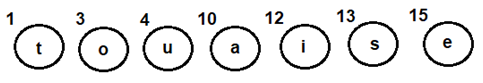 Fig 1: Leaf nodes for each character
Step B- Repeat the following steps till heap has more than one nodes
- Step 3- Extract two nodes, say x and y, with minimum frequency from the heap
- Step 4- Create a new internal node z with x as its left child and y as its right child. Also frequency(z)= frequency(x)+frequency(y)
- Step 5- Add z to min heap
- Extract and Combinenode u with an internal node having 4 as the frequency
- Add the new internal node to priority queue-
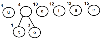 Fig 2: Combining nodes o and t
- Extract and Combine node awith an internal node having 8 as the frequency
- Add the new internal node to priority queue-
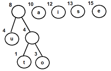 Fig 3: Combining node u withan internal node having 4 as frequency
- Extract and Combine nodes i and s
- Add the new internal node to priority queue-
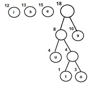 Fig 4: Combining node u withan internal node having 4 as frequency
- Extract and Combine nodes i and s
- Add the new internal node to priority queue-
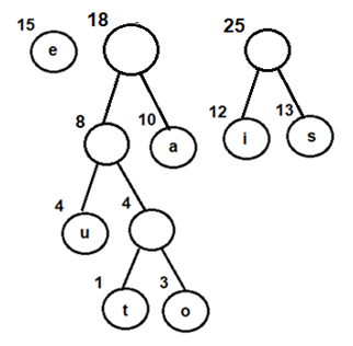 Fig 5: Combining nodes i and s
- Extract and Combine node ewith an internal node having 18 as the frequency
- Add the new internal node to priority queue-
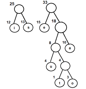 Fig 6: Combining node e with an internal node having 18 as frequency
- Finally, Extract and Combine internal nodes having 25 and 33 as the frequency
- Add the new internal node to priority queue-
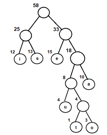 Fig 7: Final Huffman tree obtained by combining internal nodes having 25 and 33 as frequency
Now, since we have only one node in the queue, the control will exit out of the loop
Step C- Since internal node with frequency 58 is the only node in the queue, it becomes the root of Huffman tree.
Step 6- Last node in the heap is the root of Huffman tree
Steps for traversing the Huffman Tree
- Create an auxiliary array
- Traverse the tree starting from root node
- Add 0 to arraywhile traversing the left child and add 1 to array while traversing the right child
- Print the array elements whenever a leaf node is found
Following the above steps for Huffman Tree generated above, we get prefix-free and variable-length binary codes with minimum expected codeword length-
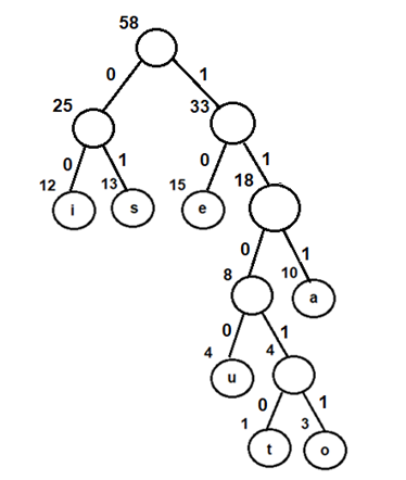 Fig 8: Assigning binary codes to Huffman tree
| Characters | Binary Codes |
| i | 00 |
| s | 01 |
| e | 10 |
| u | 1100 |
| t | 11010 |
| o | 11011 |
| a | 111 |
Suppose the string “staeiout” needs to be transmitted from computer A (sender) to computer B (receiver) across a network. Using concepts of Huffman encoding, the string gets encoded to “0111010111100011011110011010” (01 | 11010 | 111 | 10 | 00 | 11011 | 1100 | 11010) at the sender side.
Once received at the receiver’s side, it will be decoded back by traversing the Huffman tree. For decoding each character, we start traversing the tree from root node. Start with the first bit in the string. A ‘1’ or ‘0’ in the bit stream will determine whether to go left or right in the tree. Print the character, if we reach a leaf node.
Thus for the above bit stream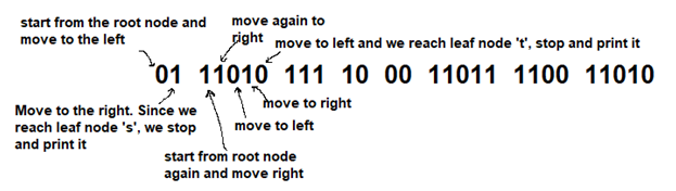 Fig 9: Decoding the bit stream
- 111 gets decoded to ‘a’
- 10 gets decoded to ‘e’
- 00 gets decoded to ‘i’
- 11011 gets decoded to ‘o’
- 1100 gets decoded to ‘u’
- And finally, 11010 gets decoded to ‘t’, thus returning the string “staeiout” back
Following is the C++ implementation of Huffman coding. The algorithmcan be mapped to any programming language as per the requirement.
#include <iostream>
#include <vector>
#include <queue>
#include <string>

using namespace std;

class Huffman_Codes
{
 struct New_Node
 {
  char data;
  size_t freq;
  New_Node* left;
  New_Node* right;
  New_Node(char data, size_t freq) : data(data),
                                 freq(freq),
left(NULL),
right(NULL)
                                 {}
 ~New_Node()
 {
   delete left;
   delete right;
 }
 };

 struct compare
 {
  bool operator()(New_Node* l, New_Node* r)
  {
    return (l->freq > r->freq);
  }
};

New_Node* top;

void print_Code(New_Node* root, string str)
{
if(root == NULL)
   return;

 if(root->data == '$')
 {
  print_Code(root->left, str + "0");
  print_Code(root->right, str + "1");
 }

 if(root->data != '$')
 {
   cout << root->data <<" : " << str << "\n";
   print_Code(root->left, str + "0");
   print_Code(root->right, str + "1");
 }
}

public:
  Huffman_Codes() {};
  ~Huffman_Codes()
  {
    delete top;
  }
  void Generate_Huffman_tree(vector<char>& data, vector<size_t>& freq, size_t size)
  {
   New_Node* left;
   New_Node* right;
   priority_queue<New_Node*, vector<New_Node*>, compare > minHeap;

for(size_t i = 0; i < size; ++i)
   {
      minHeap.push(new New_Node(data[i], freq[i]));
   }

while(minHeap.size() != 1)
    {
      left = minHeap.top();
minHeap.pop();

      right = minHeap.top();
minHeap.pop();

      top = new New_Node('$', left->freq + right->freq);
      top->left  = left;
      top->right = right;
      minHeap.push(top);
     }
    print_Code(minHeap.top(), "");
 }
};

 int main()
 {
  int n, f;
  char ch;
  Huffman_Codes set1;
  vector<char> data;
  vector<size_t> freq;
  cout<<"Enter the number of elements \n";
  cin>>n;
  cout<<"Enter the characters \n";
  for (int i=0;i<n;i++)
  {
      cin>>ch;
data.insert(data.end(), ch);
  }
  cout<<"Enter the frequencies \n";
  for (int i=0;i<n;i++)
  {
      cin>>f;
freq.insert(freq.end(), f);
  }

  size_t size = data.size();
  set1.Generate_Huffman_tree(data, freq, size);

  return 0;
}
The program is executed using same inputs as that of the example explained above. This will help in verifying the resultant solution set with actual output.
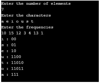 Fig 10: Output
Time Complexity Analysis-
Since Huffman coding uses min Heap data structure for implementing priority queue, the complexity is O(nlogn). This can be explained as follows-
- Building a min heap takes
O(nlogn)time (Moving an element from root to leaf node requiresO(logn)comparisons and this is done for n/2 elements, in the worst case). - Building a min heap takes
O(nlogn)time (Moving an element from root to leaf node requiresO(logn)comparisons and this is done for n/2 elements, in the worst case).
Since building a min heap and sorting it are executed in sequence, the algorithmic complexity of entire process computes to O(nlogn)
We can have a linear time algorithm as well, if the characters are already sorted according to their frequencies.
Advantages of Huffman Encoding-
- This encoding scheme results in saving lot of storage space, since the binary codes generated are variable in length
- It generates shorter binary codes for encoding symbols/characters that appear more frequently in the input string
- The binary codes generated are prefix-free
Disadvantages of Huffman Encoding-
- Lossless data encoding schemes, like Huffman encoding, achieve a lower compression ratio compared to lossy encoding techniques. Thus, lossless techniques like Huffman encoding are suitable only for encoding text and program files and are unsuitable for encoding digital images.
- Huffman encoding is a relatively slower process since it uses two passes- one for building the statistical model and another for encoding. Thus, the lossless techniques that use Huffman encoding are considerably slower than others.
- Since length of all the binary codes is different, it becomes difficult for the decoding software to detect whether the encoded data is corrupt. This can result in an incorrect decoding and subsequently, a wrong output.
Real-life applications of Huffman Encoding-
- Huffman encoding is widely used in compression formats like
GZIP, PKZIP (winzip) and BZIP2. - Multimedia codecs like
JPEG, PNG and MP3uses Huffman encoding (to be more precised the prefix codes) - Huffman encoding still dominates the compression industry since newer arithmetic and range coding schemes are avoided due to their patent issues.
Dijkstra's Algorithm
Dijkstra's algorithm, published in 1959, is named after its discoverer Edsger Dijkstra, who was a Dutch computer scientist. This algorithm aims to find the shortest-path in a directed or undirected graph with non-negative edge weights.
Before, we look into the details of this algorithm, let’s have a quick overview about the following:
- Graph: A graph is a non-linear data structure defined as G=(V,E) where V is a finite set of vertices and E is a finite set of edges, such that each edge is a line or arc connecting any two vertices.
- Weighted graph: It is a special type of graph in which every edge is assigned a numerical value, called weight
- Connected graph: A path exists between each pair of vertices in this type of graph
- Spanning tree for a graph G is a subgraph G’ including all the vertices of G connected with minimum number of edges. Thus, for a graph G with n vertices, spanning tree G’ will have n vertices and maximum n-1 edges.
Problem Statement
Given a weighted graph G, the objective is to find the shortest path from a given source vertex to all other vertices of G. The graph has the following characteristics-
- Set of vertices
V - Set of weighted edges
Esuch that(q,r)denotes an edge between vertices q and r and cost(q,r) denotes its weight
Dijkstra's Algorithm:
- This is a single-source shortest path algorithm and aims to find solution to the given problem statement
- This algorithm works for both directed and undirected graphs
- It works only for connected graphs
- The graph should not contain negative edge weights
- The algorithm predominantly follows Greedy approach for finding locally optimal solution. But, it also uses Dynamic Programming approach for building globally optimal solution, since the previous solutions are stored and further added to get final distances from the source vertex
- The main logic of this algorithm is basedon the following formula-
dist[r]=min(dist[r], dist[q]+cost[q][r])
This formula states that distance vertex r, which is adjacent to vertex q, will be updated if and only if the value of dist[q]+cost[q][r] is less than dist[r]. Here-
- dist is a 1-D array which, at every step, keeps track of the shortest distance from source vertex to all other vertices, and
- cost is a 2-D array, representing the cost adjacency matrix for the graph
- This formula uses both Greedy and Dynamic approaches. The Greedy approach is used for finding the minimum distance value, whereas the Dynamic approach is used for combining the previous solutions (dist[q] is already calculated and is used to calculate dist[r])
Algorithm-
Input Data-- Cost Adjacency Matrix for Graph G, say cost
- Source vertex, say s
- Spanning tree having shortest path from s to all other vertices in G
Following are the steps used for finding the solution-
Step 1; Set dist[s]=0, S=ϕ // s is the source vertex and S is a 1-D array having all the visited vertices
Step 2: For all nodes v except s, set dist[v]= ∞
Step 3: find q not in S such that dist[q] is minimum // vertex q should not be visited
Step 4: add q to S // add vertex q to S since it has now been visited
Step 5: update dist[r] for all r adjacent to q such that r is not in S //vertex r should not be visited dist[r]=min(dist[r], dist[q]+cost[q][r]) //Greedy and Dynamic approach
Step 6: Repeat Steps 3 to 5 until all the nodes are in S // repeat till all the vertices have been visited
Step 7: Print array dist having shortest path from the source vertex u to all other vertices
Step 8: Exit
Let’s try and understand the working of this algorithm using the following example-
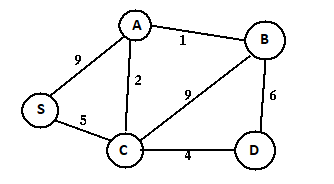 Fig 1: Input Graph (Weighted and Connected)
Given the above weighted and connected graph and source vertex s, following steps are used for finding the tree representing shortest path between s and all other vertices-
Step A- Initialize the distance array (dist) using the following steps of algorithm –
Step 1- Set dist[s]=0, S=ϕ // u is the source vertex and S is a 1-D array having all the visited vertices
Step 2- For all nodes v except s, set dist[v]= ∞
| Set of visited vertices (S) | S | A | B | C | D |
| 0 | ∞ | ∞ | ∞ | ∞ |
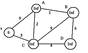 Fig 2: Graph after initializing dist[]
Step B- a)Choose the source vertex s as dist[s] is minimum and s is not in S.
Step 3- find q not in S such that dist[q] is minimum // vertex should not be visited
Visit s by adding it to S
Step 4- add q to S // add vertex q to S since it has now been visited
Step c) For all adjacent vertices of s which have not been visited yet (are not in S) i.e A and C, update the distance array using the following steps of algorithm -
Step 5- update dist[r] for all r adjacent to q such that r is not in S //vertex r should not be visited dist[r]=min(dist[r], dist[q]+cost[q][r]) //Greedy and Dynamic approach
dist[A]= min(dist[A], dist[s]+cost(s, A)) = min(∞, 0+9) = 9dist[C] = min(dist[C], dist[s]+cost(s, C)) = min(∞, 0+5) = 5
Thus dist[] gets updated as follows-
| Set of visited vertices (S) | S | A | B | C | D |
| [s] | 0 | 9 | ∞ | 5 | ∞ |
Step C- Repeat Step B by
- Choosing and visiting vertex C since it has not been visited (not in S) and dist[C] is minimum
- Updating the distance array for adjacent vertices of C i.e. A, B and D
Step 6- Repeat Steps 3 to 5 until all the nodes are in S
dist[A]=min(dist[A], dist[C]+cost(C,A)) = min(9, 5+2)= 7
dist[B]= min(dist[B], dist[C]+cost(C,B)) = min(∞, 5+9)= 14
dist[D]= min(dist[D], dist[C]+cost(C,D))= min((∞,5+4)=9
This updates dist[] as follows-
| Set of visited vertices (S) | S | A | B | C | D |
| [s] | 0 | 9 | ∞ | 5 | ∞ |
| [s,C] | 0 | 7 | 14 | 5 | 9 |
Continuing on similar lines, Step B gets repeated till all the vertices are visited (added to S). dist[] also gets updated in every iteration, resulting in the following –
| Set of visited vertices (S) | S | A | B | C | D |
| [s] | 0 | 9 | ∞ | 5 | ∞ |
| [s,C] | 0 | 7 | 14 | 5 | 9 |
| [s, C, A] | 0 | 7 | 8 | 5 | 9 |
| [s, C, A, B] | 0 | 7 | 8 | 5 | 9 |
| [s, C, A, B, D] | 0 | 7 | 8 | 5 | 9 |
The last updation of dist[] gives the shortest path values from s to all other vertices
The resultant shortest path spanning tree for the given graph is as follows-
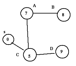 Fig 3: Shortest path spanning tree
- There can be multiple shortest path spanning trees for the same graph depending on the source vertex
Following is the C++ implementation for Dijkstra’s Algorithm
Note :
The algorithm can be mapped to any programming language as per the requirement.
#include<iostream>
using namespace std;
#define V 5  //Defines total number of vertices in the graph
#define INFINITY 999
int min_Dist(int dist[], bool visited[])
//This method used to find the vertex with minimum distance and is not yet visited
{
	int min=INFINITY,index;                 //Initialize min with infinity
	for(int v=1;v<=V;v++)
	{
		if(visited[v]==false &&dist[v]<=min)
		{
			min=dist[v];
			index=v;
		}
	}
	return index;
}
void Dijkstra(int cost[V][V],int src) //Method to implement shortest path algorithm
{
	int dist[V];
	bool visited[V];
	for(int i=1;i<=V;i++)                    //Initialize dist[] and visited[]
	{
		dist[i]=INFINITY;
		visited[i]=false;
	}
	//Initialize distance of the source vertec to zero
	dist[src]=0;
	for(int c=2;c<=V;c++)
	{
		//u is the vertex that is not yet included in visited and is having minimum
		int u=min_Dist(dist,visited);            distance
		visited[u]=true;                          //vertex u is now visited
		for(int v=1;v<=V;v++)
//Update dist[v] for vertex v which is not yet included in visited[] and
//there is a path from src to v through u that has smaller distance than
// current value of dist[v]
		{
			if(!visited[v] && cost[u][v] &&dist[u]+cost[u][v]<dist[v])
			dist[v]=dist[u]+cost[u][v];
		}
	}
	 //will print the vertex with their distance from the source
	cout<<"The shortest path  "<<src<<" to all the other vertices is: \n";
	for(int i=1;i<=V;i++)
	{
	   if(i!=src)
	   cout<<"source:"<<src<<"\t destination:"<<i<<"\t MinCost is:"<<dist[i]<<"\n";
	}
}
int main()
{
	int cost[V][V], i,j, s;
	cout<<"\n Enter the cost matrix weights";
	for(i=1;i<=V;i++)      //Indexing ranges from 1 to n
          for(j=1;j<=V;j++)
          {
cin>>cost[i][j];
			//Absence of edge between vertices i and j is represented by INFINITY
             if(cost[i][j]==0)
               cost[i][j]=INFINITY;
           }
cout<<"\n Enter the Source Vertex";
cin>>s;

	Dijkstra(cost,s);
	return 0;
}
The program is executed using same input graph as in Fig.1.This will help in verifying the resultant solution set with actual output.
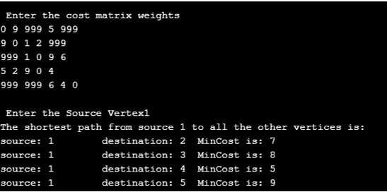 Fig 4: Output
Time Complexity Analysis-
Following are the cases for calculating the time complexity of Dijkstra’s Algorithm-
- Case1- When graph G is represented using an adjacency matrix -This scenario is implemented in the above C++ based program. Since the implementation contains two nested for loops, each of complexity O(n), the complexity of Dijkstra’s algorithm is O(n2). Please note that n here refers to total number of vertices in the given graph
- Case 2- When graph G is represented using an adjacency list - The time complexity, in this scenario reduces to O(|E| + |V| log |V|) where |E|represents number of edges and |V| represents number of vertices in the graph
Disadvantages of Dijkstra’s Algorithm-
Dijkstra’s Algorithm cannot obtain correct shortest path(s)with weighted graphs having negative edges. Let’s consider the following example to explain this scenario-
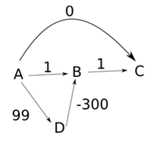 Fig 5: Weighted graph with negative edges
Choosing source vertex as A, the algorithm works as follows-
Step A- Initialize the distance array (dist)-
| Set of visited vertices (S) | A | B | C | D |
| 0 | ∞ | ∞ | ∞ |
Step B- Choose vertex A as dist[A] is minimum and A is not in S. Visit A and add it to S. For all adjacent vertices of A which have not been visited yet (are not in S) i.e C, B and D, update the distance array
dist[C]= min(dist[C], dist[A]+cost(A, C)) = min(∞, 0+0) = 0
dist[B] = min(dist[B], dist[A]+cost(A, B)) = min(∞, 0+1) = 1
dist[D]= min(dist[D], dist[A]+cost(A, D)) = min(∞, 0+99) = 99
Thus dist[] gets updated as follows-
| Set of visited vertices (S) | A | B | C | D |
| [A] | 0 | 1 | 0 | 99 |
Step C- Repeat Step B by
- Choosing and visiting vertex C since it has not been visited (not in S) and dist[C] is minimum
- The distance array does not get updated since there are no adjacent vertices of C
| Set of visited vertices (S) | A | B | C | D |
| [A] | 0 | 1 | 0 | 99 |
| [A, C] | 0 | 1 | 0 | 99 |
Continuing on similar lines, Step B gets repeated till all the vertices are visited (added to S). dist[] also gets updated in every iteration, resulting in the following –
| Set of visited vertices (S) | A | B | C | D |
| [A] | 0 | 1 | 0 | 99 |
| [A, C] | 0 | 1 | 0 | 99 |
| [A, C, B] | 0 | 1 | 0 | 99 |
| [A, C, B, D] | 0 | 1 | 0 | 99 |
Thus, following are the shortest distances from A to B, C and D-
A->C = 0 A->B = 1 A->D = 99
But these values are not correct, since we can have another path from A to C, A->D->B->C having total cost= -200 which is smaller than 0. This happens because once a vertex is visited and is added to the set S, it is never “looked back” again. Thus, Dijkstra’s algorithm does not try to find a shorter path to the vertices which have already been added to S.
- It performs a blind search for finding the shortest path, thus, consuming a lot of time and wasting other resources
Applications of Dijkstra’s Algorithm-
- Traffic information systems use Dijkstra’s Algorithm for tracking destinations from a given source location
- Open Source Path First (OSPF), an Internet-based routing protocol, uses Dijkstra’s Algorithm for finding best route from source router to other routers in the network
- It is used by Telephone and Cellular networks for routing management
- It is also used by Geographic Information System (GIS), such as Google Maps, for finding shortest path from point A to point B


0 Comments